


Most modern oscilloscopes belong to the digital storage oscilloscope (DSO) family. Most of the concepts introduced in this guide are specific to DSO.

What is an oscilloscope?
An oscilloscope is a test & measurement instrument that rapidly measures voltage over time. It records the voltage across certain points in a circuit and displays voltage (Y-axis) as a function of time (X-axis) on a screen. It is essentially a very fast voltmeter with the capability of data-logging and plotting (Figure 1).
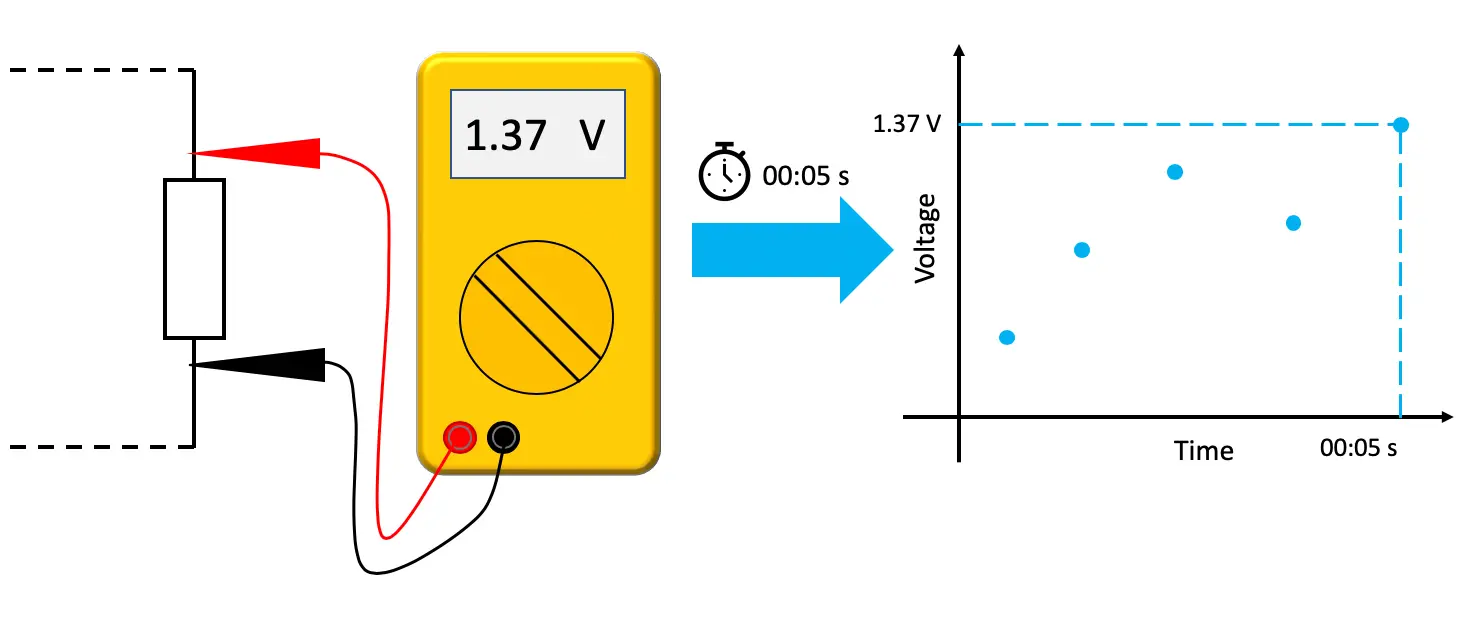
Figure 1: An oscilloscope can be considered a fast voltmeter that measures voltage at given time intervals, then logs and displays the voltage trace as a function of time.
One of the key characteristics of an oscilloscope is the speed at which it can measure and record the voltage. On a specification sheet, it is called sampling rate. The sampling rate of an oscilloscope is typically measured by the number of points it can measure over a second. For example, the Moku:Lab’s oscilloscope has a maximum sampling rate of 500 MSa/s. That is 500,000,000 measurements in a second. The MSa/s stands for mega-samples (106) per second. In theory, the highest frequency an instrument can measure is limited to ½ of the sampling frequency. This is called the Nyquist condition. However, in most cases, the sampling rate is not the limiting factor of an oscilloscope. The bandwidth of the oscilloscope describes the highest frequency the analog input can handle. It is usually described by the cut-off frequency with -3 dB attenuation. Signals significantly beyond the cut-off frequency are attenuated. The sampling rate and bandwidth combined is the defining specification of an oscilloscope. The sampling rate is typically designed around the bandwidth. Modern oscilloscopes have sampling rates ranging from hundreds of mega-samples to tens of giga-samples per second (109), and bandwidths ranging from tens of MHz to a few GHz. Higher sampling rates and bandwidth usually provide better signal modality, though that comes at a price. As a rule of thumb, the bandwidth of the oscilloscope should be at least 3 to 5 times larger than the fundamental frequency of the signal you wish to measure. To capture a sharp rising/falling feature, such as a square wave that comprises many sine waves of different frequencies, larger bandwidth is necessary.
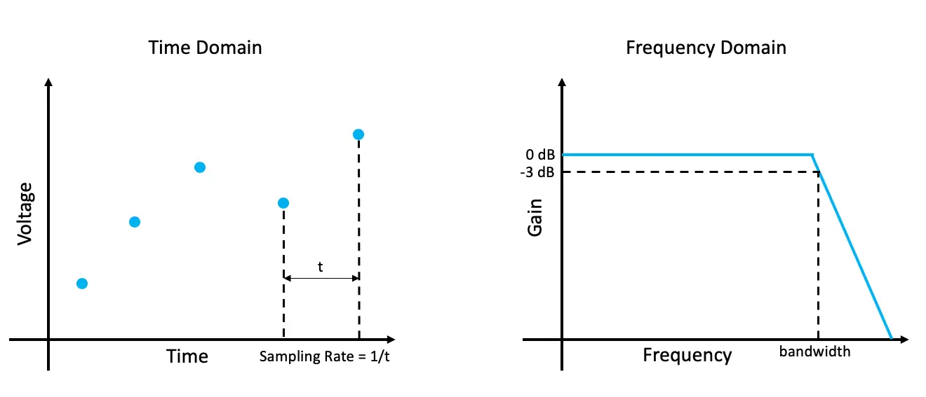
Figure 2: Two most important specifications of an oscilloscope: sampling rate and bandwidth.
Input settings
We have covered the basic function and two key specifications of an oscilloscope. Now, we will examine some details. First, the input settings. Most oscilloscopes have either two or four input channels. Channels can be individually turned on, turned off, and configured. The input settings change how the analog front ends are configured, which mainly affects the Y-axis on the display. The three most important input settings for Moku:Lab’s oscilloscope are: vertical scale (input range), coupling, and impedance.
Vertical Scale:
The scale determines the voltage range on the Y-axis. Digital storage oscilloscopes typically have limited vertical resolution (number of points they can use to represent the full input range). It is a good practice to use the entire input range when possible. The vertical scale in an oscilloscope is typically directly associated with the input gain. Once you have the signal displayed on your scope, adjust the vertical scale accordingly to ensure the signal is neither saturated nor underfilled.
Coupling:
The input coupling determines which part(s) of your signal (DC and AC) pass through the input. In DC coupling, both DC and AC components pass through the input. In AC coupling, only the AC component is allowed through the input. This is useful when you want to probe a small AC oscillation on top of a large DC offset. The cut-off frequency for AC coupling is typically around 50-60 Hz.
Impedance:
The impedance determines the resistance of the input load resistor. Most oscilloscopes have the option to choose between 50 Ω or 1 MΩ. Selection depends upon the source impedance of the signal. Typically 1 MΩ is used to measure voltages accurately because it disrupts the input signal less, while 50 Ω is used to measure power at high frequencies and to connect to other devices with 50 Ω impedances.
Oscilloscopes often use probes to connect with electrical circuits and these can typically be 1x or 10x probes. 1x probes pass through the signal with no amplitude scaling, where 10x probes provide a resistor divider that scales the signal by 1/10th. A 1x or 10x probe-type can also be set in the Moku:Lab input settings, so that the display correctly reflects the probe scaling and actual signal magnitude.
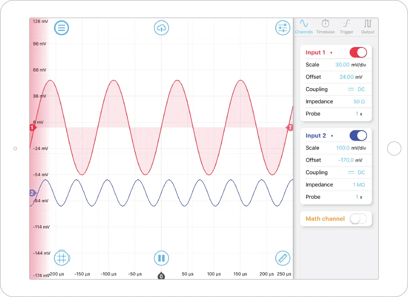
Figure 3: Input settings for Moku:Lab’s Oscilloscope. You can adjust the vertical scale, change the input coupling, and change the input impedance for your scope.
Trigger function
The trigger function is one of the most important mechanisms in an oscilloscope. As we discussed in the previous section, the sampling rate of an oscilloscope is several hundred MHz to several GHz. In practice, it is impossible to display and store that number of data points continuously on the screen. That’s where the trigger mechanism comes into play. Instead of continuously capturing data, the scope captures a certain number of data points (i.e. 10,000 points) after it is “triggered”. Once triggered, the scope displays these 10,000 points on the screen, then waits for the next trigger. If the trigger events happen faster than what the scope can handle, it will just ignore these intermediate triggers until the oscilloscope is ready for the next trigger. This means the waveforms displayed on the screen may not be consecutive in time. Instead, the scope continuously displays these “snapshots” captured at each trigger event (Figure 4). Most oscilloscopes have a “roll” mode, which continuously captures and displays the data points without a trigger. However, the sampling rates used for roll mode are typically much slower.
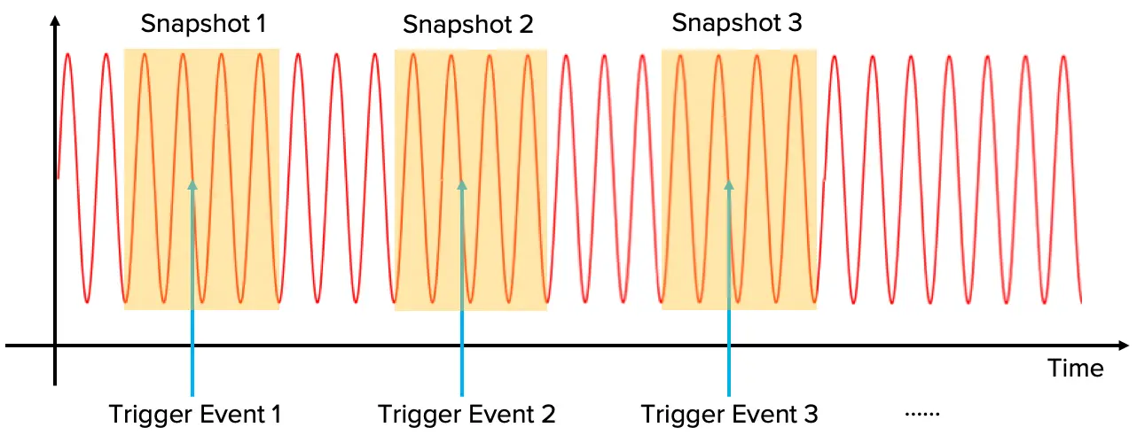
Figure 4: Oscilloscopes display snapshots of trigger events on the screen. If the trigger event happens faster than the scope can handle, the waveforms displayed are not consecutive in time.
Trigger Condition:
The oscilloscope is typically triggered when the voltage on one of the input channels rises / falls across a certain level. For example, we can trigger the scope when the voltage on input 1 rises across 1 V. The triggering condition is highly customizable, and some oscilloscopes have more advanced trigger conditions. However, we will not cover them in this introductory tutorial.
Trigger Mode:
In most oscilloscopes, there are three different trigger modes: “Auto”, “Normal”, and “Single”. In the “Auto” mode, a “force” trigger happens when the scope does not detect a trigger event after a certain amount of time. The scope will always display the latest-acquired data, even if the trigger condition is not met. In “Normal” mode, the scope is only triggered when the set trigger condition is met. The scope will always wait for the next trigger event, instead of applying a “force” trigger. In “Single” mode, the oscilloscope waits for the next trigger event. Once it’s triggered, it will pause the screen and display the waveform captured with that trigger.
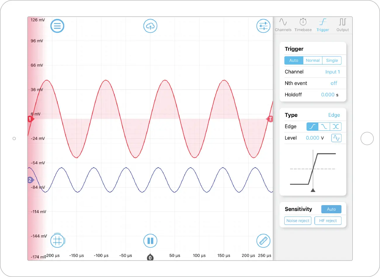
Figure 5: Trigger settings for Moku:Lab’s oscilloscope. You can select between auto, normal, and single trigger mode. Also, you can customize the trigger condition based on your measurement.
Timebase (horizontal scale)
Now we will discuss the X-axis. The timebase of the oscilloscope controls the behavior of the horizontal axis. By adjusting the timebase, the oscilloscope will automatically choose an optimal sampling rate that balances the length of the trace (in time) and time resolution. Why don’t we always use the maximum sampling rate? As we mentioned previously, the number of points the scope can store per trigger event is limited by its internal memory. Let’s say the sample size is 10,000 points. If the signal we want to observe is oscillating at 1 Hz, then at 500 MSa/s, 10,000 points displays 0.000002 second of data. At that rate, we cannot get anywhere close to the full picture of the 1 Hz signal! So, the sampling rate needs to be optimized when we adjust the scale of the X-axis. The lower the frequency being analyzed, the longer the time base and the wider the gap between sample presented.
A DSO has a finite sampling rate. This means the data points acquired by the scope are not truly continuous in time. To display a continuous waveform on screen when zooming in on the time axis, different interpolation modes can be selected. Linear interpolation does not perform any up-sampling. To display a waveform, a straight line is drawn between consecutive points. This is “ugly” but doesn’t “invent” any new data points. SinX/X interpolation preserves the frequency characteristics of the signal. In the time domain though, it can appear that there is over- or under-shoot that is not in fact present in the signal. Gaussian interpolation “smooths” the signal out, preserving the time domain visual characteristics of the signal at the expense of frequency information.
If the waveform you are trying to capture is repetitive for each trigger event, it is sometimes useful to average several trigger events and display the averaged waveform. This should significantly improve the signal-to-noise ratio of a relatively weak signal.
Persistence setting allows you to keep the given number of old waveforms (trigger events) on the screen. It helps to observe changes of waveforms over time.
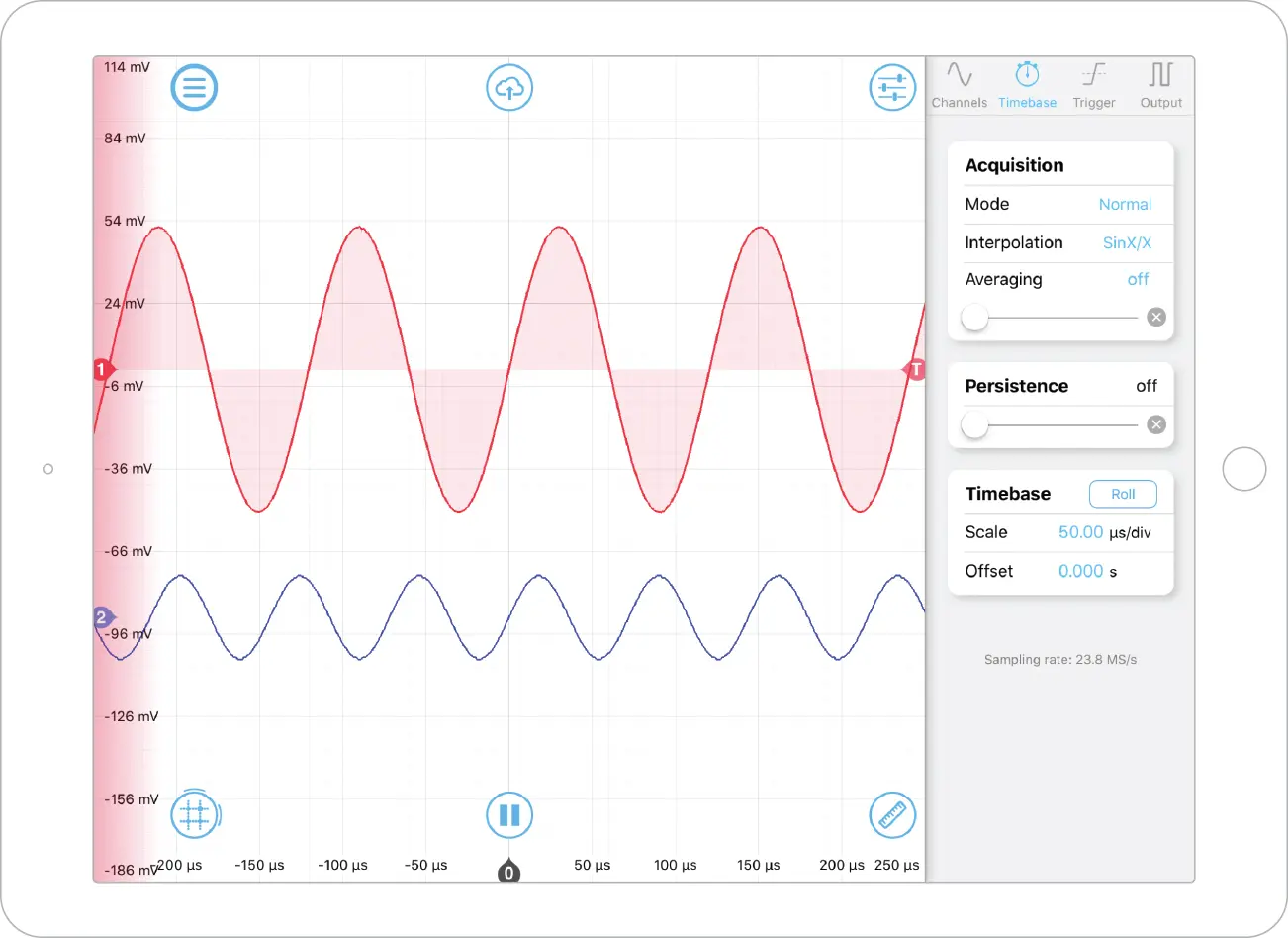
Figure 6: Timebase settings for Moku:Lab’s oscilloscope. The sampling rate is automatically determined by the horizontal scale.
Advanced features
Now we will talk about some of the automated functions built into the oscilloscope. A modern oscilloscope can measure various properties of captured waveforms such as amplitude, frequency, etc. So instead of calculating the frequency of the input waveform by counting the time interval on your screen, you can make the scope do the calculation automatically for you. Most oscilloscopes also have math functions such as: add, subtract, and even perform Fast Fourier Transform (FFT) analysis on the input waveforms. All these functions combined make modern oscilloscope a really practical tool to have in the lab for analyzing circuits, communication signals, etc.
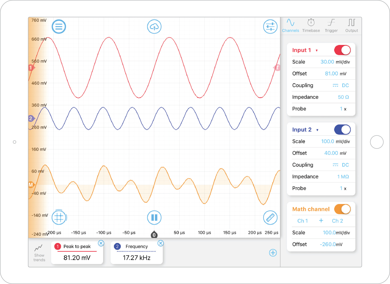
Figure 7: The math and measurement function of Moku:Lab’s oscilloscope. The orange trace shows the sum of Input 1 and Input 2. The peak to peak measurement of Input 1, and the frequency measurement of Channel 2 are displayed on the bottom of the signal display area.
Thanks for reading this oscilloscope familiarization guide. You can download the Moku:Lab App from Apple’s App Store and experience it in demo mode. Details about specific features of Moku:Lab’s Oscilloscope can be found in the Oscilloscope User Manual.
Have questions or want a printable version?
Please contact us at support@liquidinstruments.com