Moku:Go’s Arbitrary Waveform Generator

Using MATLAB to generate modulated arbitrary waveforms

April 19, 2021

Arbitrary waveform generators are used to output specific stimulus signals for a device under test, such as detectors and communication devices. In this application note, we provide a tutorial on using Moku:Go’s Arbitrary Waveform Generator with MATLAB to generate two arbitrary waveforms with pulse and burst modulation.

The MATLAB script and text file accompanying this note are available to download from the Liquid Instruments website.

Moku:Go

Moku:Go combines 14+ lab instruments in one high performance device, with 2 analog inputs, 2 analog outputs, 16 digital I/O pins and optional integrated power supplies.

Arbitrary Waveform Generator

Detectors and communication devices generally work with highly arbitrary signals, rather than standard sine waves and square waves. Characterizing such devices, therefore, requires an arbitrary waveform generator (AWG), which can output user-defined waveforms to simulate specific signals for the device under test. The waveforms can be based on mathematical formulas or from pre-recorded data. For example, to test an earthquake detector, engineers can generate a pre-recorded earthquake signal and analyze the detector’s response and refine the detector design accordingly.

Moku:Go’s Arbitrary Waveform Generator can generate custom waveforms with up to 65,536 points at sampling rates of up to 125 MSa/s. Waveforms can be loaded from a file, or input as a piece-wise mathematical function with up to 32 segments, to generate truly arbitrary waveforms.

Aside from the capability of generating user-defined waveforms, Moku:Go’s AWG also has two modulation modes: pulse and burst. Pulse modulation repeats the signal at a much slower rate and allows for the signal to
hold a set voltage between cycles. Pulse mode is used for simulating low-duty cycle repetitive events, such as radar detectors that emit a signal and measure the returned signal. Burst mode generates the output once the trigger condition is met. This can be the impulse response of a particle counter or the response of a digital communication device. Signal modulation, therefore, enables AWGs to be used in an even wider range of applications.

In this note, we will utilize the Moku application programming interface (API) for MATLAB to generate two different waveforms from the Moku:Go and measure the output signals with another Moku:Go using the Windows Moku:Go App. We will demonstrate how to load a signal from a text file and how to generate one based on a mathematical formula. We will then apply pulse modulation and burst modulation to each signal.

This note is accompanied by the example script AWG_appnote.m and the text file containing the custom
waveform sq_wave.txt available at https://download.liquidinstruments.com/documentation/app-note/referencefiles/Using_AWG_with_Moku_Go_Supporting_Files.zip

Please also make sure to have the Moku-MATLAB Toolbox installed before running the example script, the toolbox can be downloaded from:

https://www.liquidinstruments.com/resources/software-utilities/matlab-api/.

Generating custom waveforms

In this section, we will generate the two waveforms using Moku:Go’s AWG. The two waveforms are shown in Figure 1: a square wave and a chirp signal.

The square wave is an array of 1000 elements and is loaded from the accompanying text file sq_wave.txt. This is not only for demonstrating how a custom waveform can be loaded from a file but also to show an example waveform definition file that can be used for Moku:Go AWG, as the same file can also be used in the Windows and Mac App.

The second waveform is also an array of 1000 elements and is generated using the following equation:

y = sin[2π(50t²)]

where t is an array of 1000 elements evenly spaced from 0 to 1. Moku:Go AWG only requires the voltage values to form its lookup table, t is only used for calculating y values and generating the plot in Figure 1.

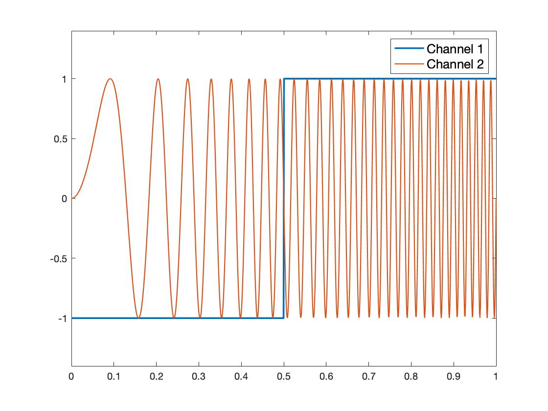
Figure 1: MATLAB plot of example waveforms

Once the arbitrary waveforms are loaded into the lookup table, we can deploy them to the Moku:Go and start generating signals.

The connection to Moku:Go is established via its IP address using the following MATLAB command at line 30 of AWG_appnote.m.

m = MokuArbitraryWaveformGenerator(ip, true);

Replace ip with the IP address of your Moku:Go to connect to the device.

The output waveforms are then set using the generate_waveform command, which takes in five required parameters in this order: channel, sample rate, lookup table data, frequency, and amplitude. For example, output channel 1 is set at line 39 as the following:

m.generate_waveform(1, "Auto", square_wave, le3, 1);

This means channel 1 will generate a signal at an automatically assigned sample rate using the square_wave lookup table. The signal will have a frequency of 1kHz and an amplitude of 1V_pp.

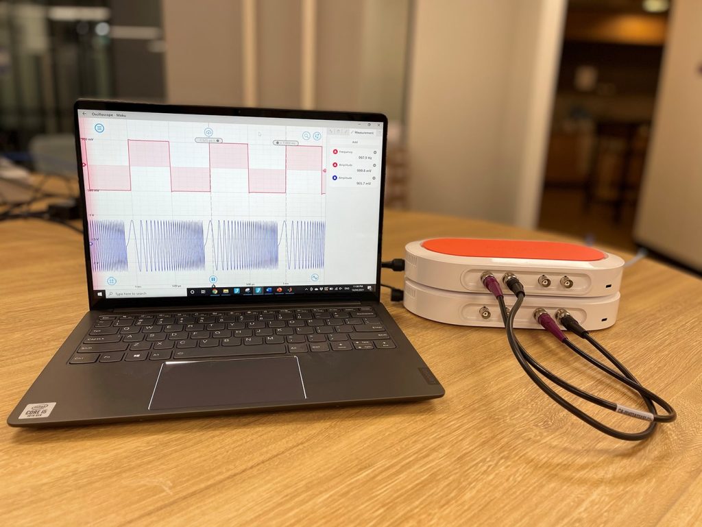
Figure 2: Moku:Go measurement hardware setup

To confirm that the output signals from the AWG match the waveforms in Figure 1, we set up another Moku:Go running the Oscilloscope instrument using the Windows App interface. In Figure 2, the top Moku:Go is running the Oscilloscope instrument, while the bottom Moku:Go is running the AWG instruments. The outputs of the Moku:Go running the AWG are connected to the inputs of the Moku:Go running the Oscilloscope.

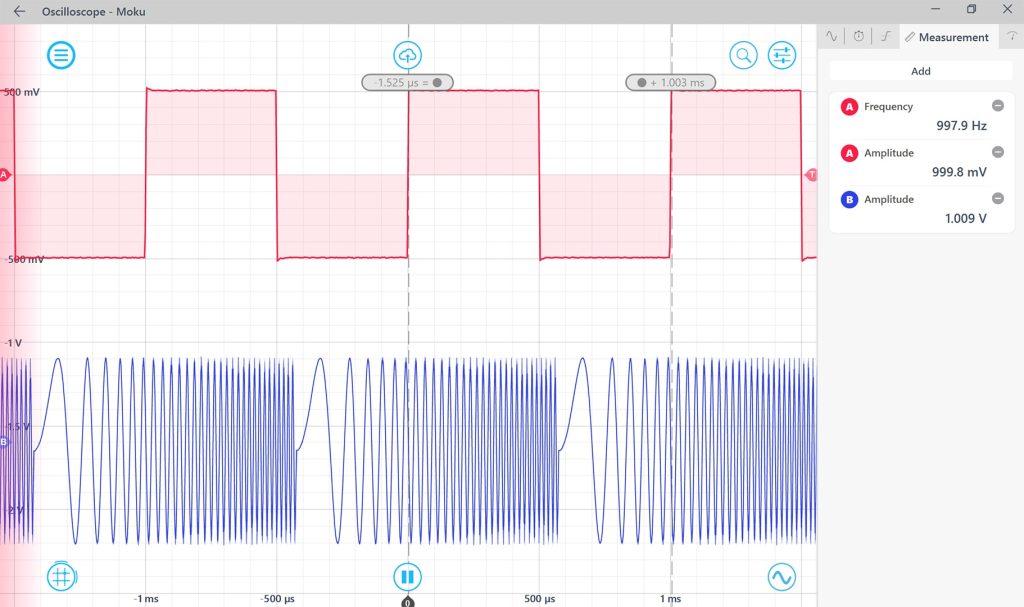
Figure 3: Moku:Go Oscilloscope measuring the AWG output generated from the MATLAB example script.

The captured signals are shown in Figure 3, which matches the waveforms in Figure 1. Channel 1 of the Oscilloscope measures the frequency as expected to be 1kHz (actual measurement is 998.4 Hz). This is also confirmed with the cursors, here the period of 1 cycle of the square wave is 1ms. The amplitudes of both channels measure 1V_pp as expected (actual measurement 0.9998V for Channel 1 and 1.009V for Channel 2).

Pulse modulation

In pulse modulation mode, the output waveform can be configured to have up to 2¹⁸ = 262144 cycles of dead time between each repetition of the arbitrary waveform.

In this example, we will introduce 2 dead cycles in the square wave signal using pulse modulation.

Pulse modulation can be switched on in the example script by uncommenting line 51 in the pulse modulation section. The modulation properties are configured as:

m.pulse_modulate(1, 'dead_cycles',2,'dead_voltage',0);

where the first parameter is the channel to apply pulse modulation to; 2 cycles of dead time are between each cycle of the signal; the voltage during dead time is 0V.

The waveform is also confirmed using the Oscilloscope in Figure 4.

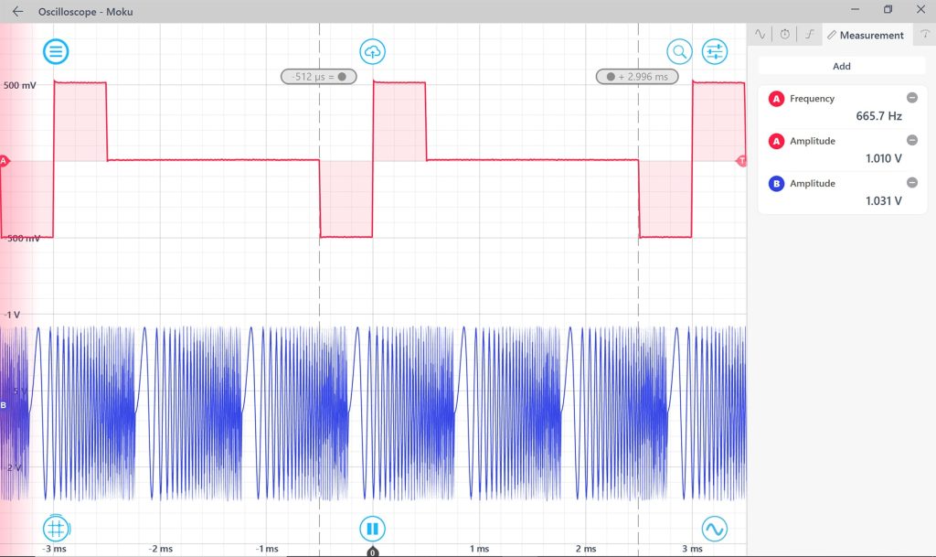
Figure 4: Square wave with pulse modulation measured by the Oscilloscope.

Burst modulation

In burst mode, the output waveform can be triggered from another signal source. Once the trigger condition is met, the signal will be generated with set burst conditions. Moku:Go offers two types of burst modes: NCycle enables a set number of cycles of the waveform to be generated when triggered; Start will start the waveform output when triggered.

In this example, we will generate a square wave (1 V_pp 200 Hz) using the Oscilloscope Moku:Go (top unit) with the built-in Waveform Generator. This square wave will be fed into Input 1 of the AWG Moku:Go (bottom unit) as the trigger signal for burst modulation.

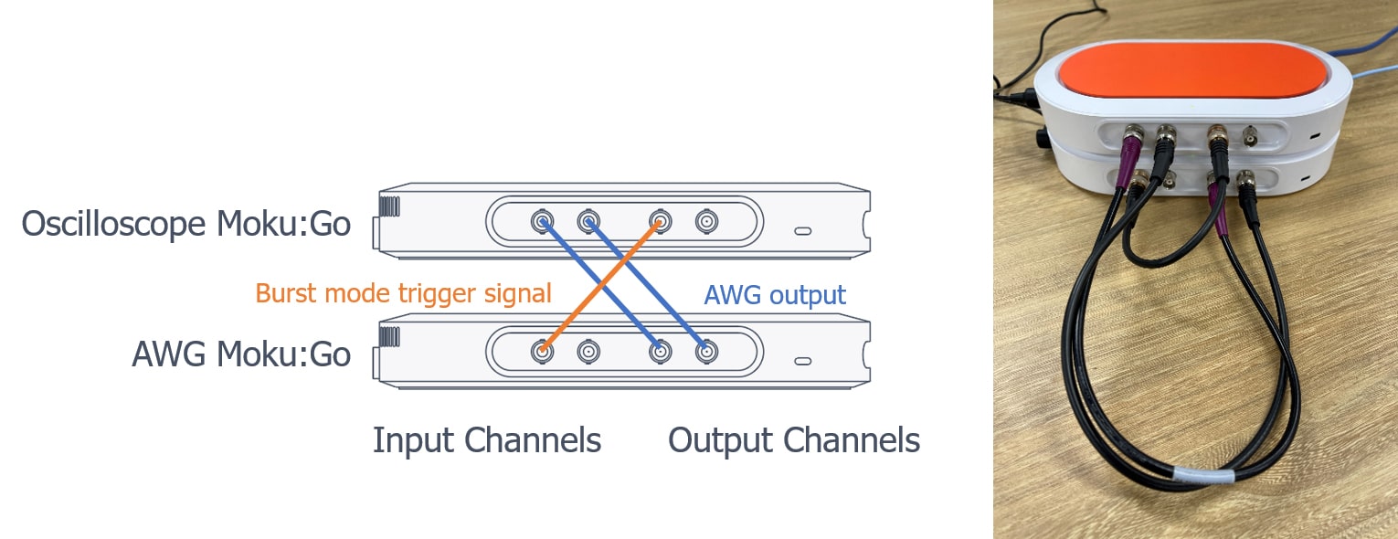
Figure 5: Moku:Go hardware setup with Oscilloscope Output 1 as the trigger signal for the AWG

Burst modulation can be enabled in the example script by uncommenting line 58 of the example script. The modulation is configured as:

m.burst_modulate(2,'Input1','NCycle','burst_cycles',2,'trigger_level',0.1);

where output channel 2 is triggered by input 1 and will generate 2 cycles of the chirp signal once triggered. The trigger condition is when the output 1 signal crosses 0.1 V with a rising edge. A trigger level of 0.1 V is chosen as it is a sharp rising edge in the square wave to create a clear trigger.

Figure 6 shows the signal captured by the Oscilloscope, where channel 1 has been set to display the trigger signal. We can see that for every cycle of the square wave, 2 cycles of the chirp waveform are generated from the AWG.

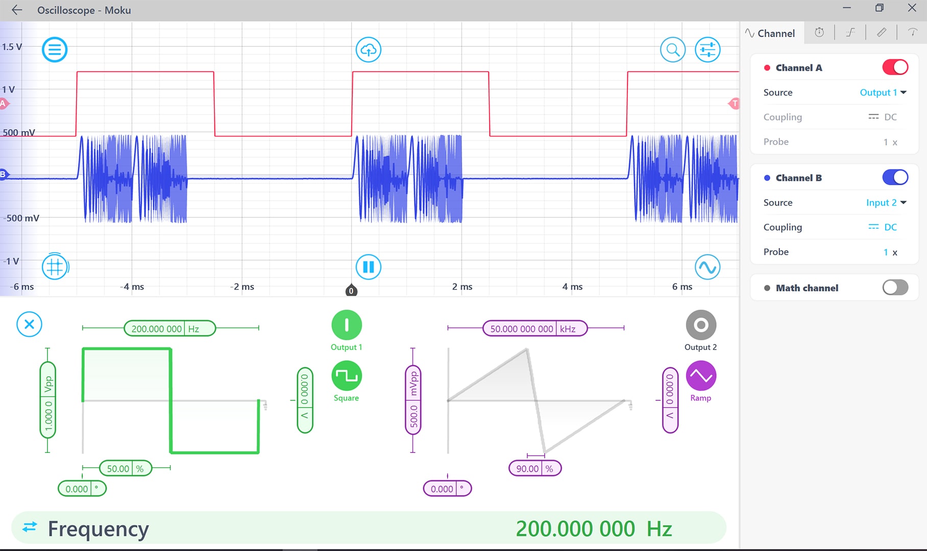
Figure 6: Burst modulated chirp signal with the Oscilloscope output square wave as trigger.

Summary

This application note has shown the flexibility with which you can define a waveform in Moku:Go’s Arbitrary Waveform Generator using MATLAB. Whether the waveform is defined by a mathematical formula or loaded from a file, the same MATLAB script can seamlessly download the waveform to Moku:Go and configure the instrument.