Moku:Go combines 15+ lab instruments in one high performance device. This application note uses Moku:Go’s PID Controller, Oscilloscope, and Programmable Power Supplies to provide a visually engaging way of learning various tuning methods for PID controllers.

Moku:Go

Moku:Go combines 15+ lab instruments in one high performance device, with 2 analog inputs, 2 analog outputs, 16 digital I/O pins and optional integrated power supplies.

PID Controller
The Proportional-Integral-Derivative (PID) controller is one of the most common forms of feedback control that is used in a wide variety of applications like the cruise control in your car or motor control in a flying drone. The purpose of a PID controller is to drive a process to reach a specified output, typically called a setpoint. The feedback of the controller is used to regulate and optimize the control of this process.
The purpose of this application is to introduce Moku:Go’s PID controller and how it can be easily integrated into a lab environment to teach control theory. Typically, control theory is taught primarily through rigorous mathematical modeling and computation, with the few labs for the class being centered around controlling the temperature of an object or the speed of a DC motor. This note introduces a modern approach to control theory education by applying a more visual component that helps students more readily connect the theory learned in the classroom to physical control systems. This is realized by controlling the height of a ping-pong ball by using a DC motor fan, an IR distance sensor, and a Moku:Go. The Moku:Go contains an integrated Oscilloscope, PID Controller, Waveform Generator and Programmable Power Supplies that can drive the motor control circuitry, take in sensor data, and output a specified signal to control the DC motor’s speed. This way, differences between when the PID controller is implemented, and when it is not, can be easily spotted by comparing characteristics like the rise time, overshoot, and steady-state height of the ping-pong ball between implementations. It also allows real-time tuning through the Moku: app so that students can see how the different PID gains impact the system both mathematically and physically. The full component list for this lab can be found in the Experimental Setup section below.
Experimental setup
Components
- Moku:Go [x1]
- 5 V Fan [x1]
- Polycarbonate tubing [~100cm]
- IC3 GP2Y0A21YK IR Distance Sensor [x1]
- IC1 NE555 (timer), IC2 LM358 (op-amp) [x1]
- Q1 IRFZ44N (MOSFET), Q2 C1815 (transistor) [x1]
- D1 1N4004 (diode) [x1]
- C1 200nF [x1], C2 47nF [x1], C3 330μF [x1]
- R1 27kΩ [x1], R2 39kΩ [x1], R3 120kΩ [x1], R4/R5/R6 10kΩ [x3] resistors
- 50kΩ potentiometer
- Breadboard [x1]

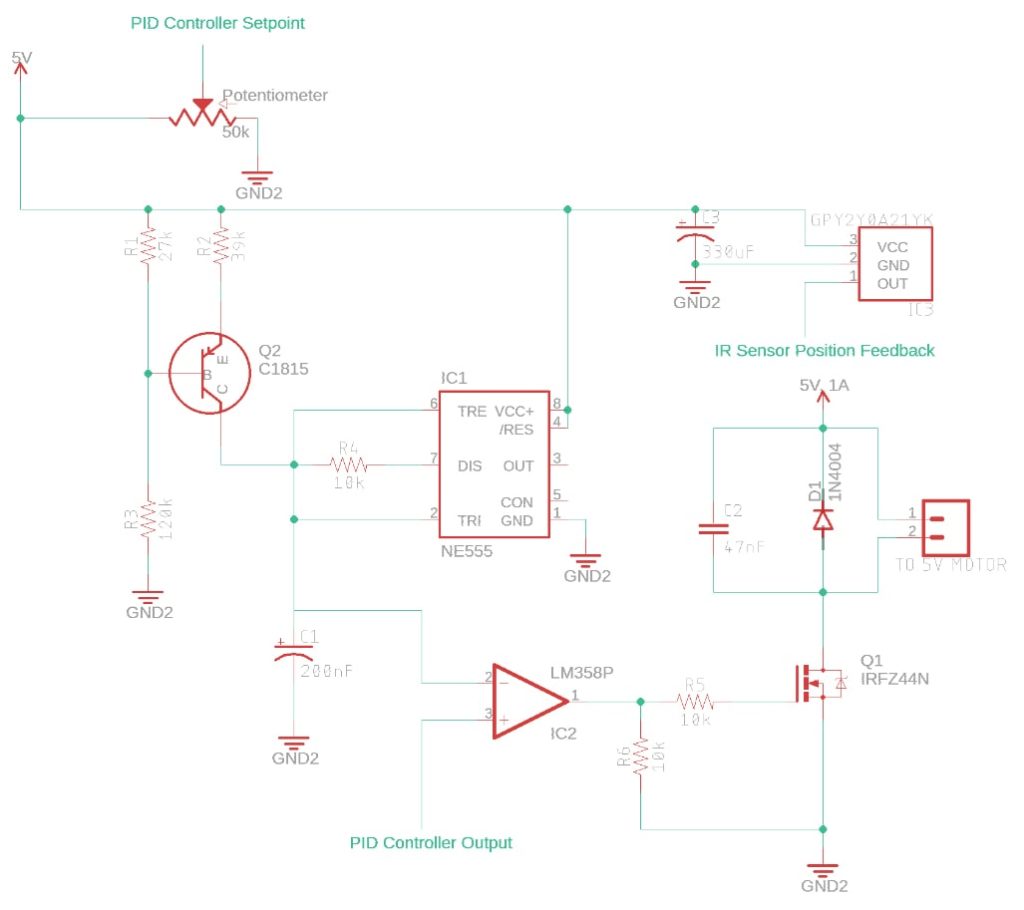
Figure 1: PWM-based DC Motor Speed Control Schematic
The circuit above is using the NE555 timer (IC1) to generate a sawtooth waveform which is fed into the inverting input of the comparator (IC2). The PID controller’s output from Moku:Go (Output 1) is fed into the non-inverting input of the comparator, which generates a PWM signal. This signal is sent to a MOSFET (Q1) that controls the power consumed by the 5V fan. The amount of power the fan sees directly translates to the height that the ping-pong ball will levitate. The way to control the height is by using the setpoint potentiometer that is connected to the Moku:Go through Input 1. This setpoint is what the PID controller uses to determine what the DC voltage on Output 1 should be to get the desired height of the ping-pong ball. For closed loop control of the ball’s height, connecting the output of the IR sensor (IC3) to Input 2 of Moku:Go and reconfiguring the control matrix of the PID allows for improved response time to changes in the setpoint from the potentiometer. A schematic showing Moku:Go’s connections can be seen below in Figure 2.

Figure 2: Schematic with Moku:Go Connections

Figure 3: Fan with Polycarbonate Tubing, IR Sensor, and Ping-Pong Ball
The other part of this lab setup is the mechanical system that is being used to levitate the ping-pong ball in the air. It consists of a 5V fan, polycarbonate tubing, IR sensor, and a ping-pong ball. The tubing is fitted to the output of the fan with some rubber strips and markings are placed every 5cm for easy measurements. It is important to note the tubing has three ¼ inch holes at each 5cm level to give the system “resistance”. This is important to the setup, otherwise the ball will float to the top every time the fan is turned on, regardless of the amount of power sent to the fan. The IR sensor is placed at the top of the tube such that as the ball rises, the voltage output from the sensor also rises.
PID Controller Model
We want to control the height of a ping-pong ball and we want to use a PID controller to do so, which means we need to find the P, I, and D gains that optimize our system for the process we want it to accomplish. However, we must first understand our system mathematically and see how the PID controller effects our system before we can plug in values for our PID gains. From control theory, we know that a PID controller can be modeled as the transfer function shown below where C(s) is the controller transfer function, G(s) is the plant transfer function, R is the reference, e is the error (e = R – Y), and Y is the output of the system.

Figure 4: Block diagram with PID controller
Using our knowledge of control theory, we know that…

… where KP is the proportional gain, KI is the integral gain, and KD is the derivative gain. These gains are what we need to find in order to optimize the rise time, settling time, overshoot, and steady-state error of our system. The table below shows how increasing each of the PID gains changes each of these system characteristics. Decreasing the gains would have the opposite effect of that shown in the table.

Table 1: PID Tuning Parameters
This table comes in handy when fine-tuning a PID controller after the gains have been found, or if you are using a “trial-and-error” method to design a controller. However, there is another method that will give us fairly good PID gain values just by analyzing the open loop step response of the system. This is known as the Ziegler-Nichols method which is commonly taught in control systems courses and can be used to quickly find starting PID gain values and then fine tune the controller afterwards using Table 1. The following shows a quick and seamless way to use Moku:Go’s PID Controller and Oscilloscope to implement the Ziegler-Nichols method and then fine tune the controller in real-time using the Moku:Go desktop app.
Ziegler-Nichols Method
The Ziegler-Nichols tuning method uses the transient step response of an open loop system to determine initial PID parameters for PID controller. These values are not perfect for every system and the controller should still be verified and tuned afterwards, however, it provides a solid starting point for most control systems. This method will only work for a system in which its open loop step response resembles that of an S-shaped curve, like the one shown in Figure 5 below, which means it has no complex-conjugate poles.

Figure 5: Ziegler-Nichols Reaction Curve
The ping-pong ball system resembles a first order, translating mass type system that typically has a transfer function of:

…where m is the mass of the ball and b is a coefficient of friction which is being modeled by holes in the tubing that the ping-pong ball is enclosed in. Without the holes in the tube, there would be no opposing force and the ball would shoot straight to the top every time the fan is turned on, no matter the power applied.
Using the Oscilloscope instrument in the Moku: app (Windows/MacOS), we can capture the IR sensor’s output as the ping-pong ball rises due to the step input. The step input is being applied to the non-inverting input of the op-amp which is connected to Output 1 of Moku:Go. This step input is being translated to a PWM signal that drives the fan motor, so it is necessary to find an appropriate step input voltage for the desired height that the ball will be tuned for. In this case, I am setting my step input to 1.950V, which translates to a 50% duty cycle and a ball height of 40cm. This may vary between systems depending on the components you choose and variance in weight of the ping-pong ball.

Figure 6: Open Loop Step Input Response
A few things to note about Figure 6 – The 960.7mV offset is expected from the IR sensor and will vary depending on the length of the tube. For this application, the tubing is 60cm long, so the offset will be the voltage the IR sensor datasheet says the output will be when an object is 60cm away (assuming the IR sensor is at the top of the tube). The pop-up at the bottom of the screen is the Oscilloscope’s built-in Waveform Generator, which allows you to use both the Oscilloscope and Waveform Generator instruments at the same time. This allows easy characterization of the step input response since we can quickly change the step input (the 1.950V DC signal) and measure the step input all from the same screen. Finally, the pop-up on the right side of the screen is the measurements tab that contains 24 unique measurements including rise time, overshoot, undershoot, and more.
We can quickly characterize the step input response by using the built-in measurements tab and applying the Ziegler-Nichols tuning method. There is no way to add a tangent line to the inflection point on the graph while in the app, however by using the High level and Low level measurements in conjunction with a few voltage and time cursors, we can approximate the time delay L and the time constant T. The time delay L is the time from when the step input is applied to when the system reacts to the step input, which is 2.645s in this case. The time constant T is the time it takes for the response to occur and is 0.58s in this case. The time constant should be fairly close to the rise time shown in the measurements tab on the right.
The method for finding these constants is by using a long straight object, like a ruler, and simply holding it up to the inflection point on the screen and then dragging two time cursors to where the ruler intersects the High level and Low level voltage cursors. The easiest way to apply the cursors is by dragging them in from the bottom left cursor icon. Click and drag up for time cursors and drag right for voltage cursors. The last step is to apply a reference time cursor to when the step input was applied, which was at -2.831s here. The reason the reference cursor is negative is because the trigger is set to a single acquisition mode such that when the IR sensor’s output voltage crosses the trigger threshold, the signal is centered to 0s on the Oscilloscope’s screen.
After using the cursors to calculate the time delay L and time constant T, we can now calculate the PID controller gains using Table 2 below.

Table 2: Ziegler-Nichols Tuning Parameters
The last step before putting these values into the PID controller is to convert them to decibels, which can be done using the equation…

…where Kdb is the gain in decibels and Kn is the gain calculated from Table 2 above.
At this point, we can enter the PID gains into the PID Controller instrument of Moku:Go by clicking on the controller box in one of the two signal chains shown in Figure 7 below.
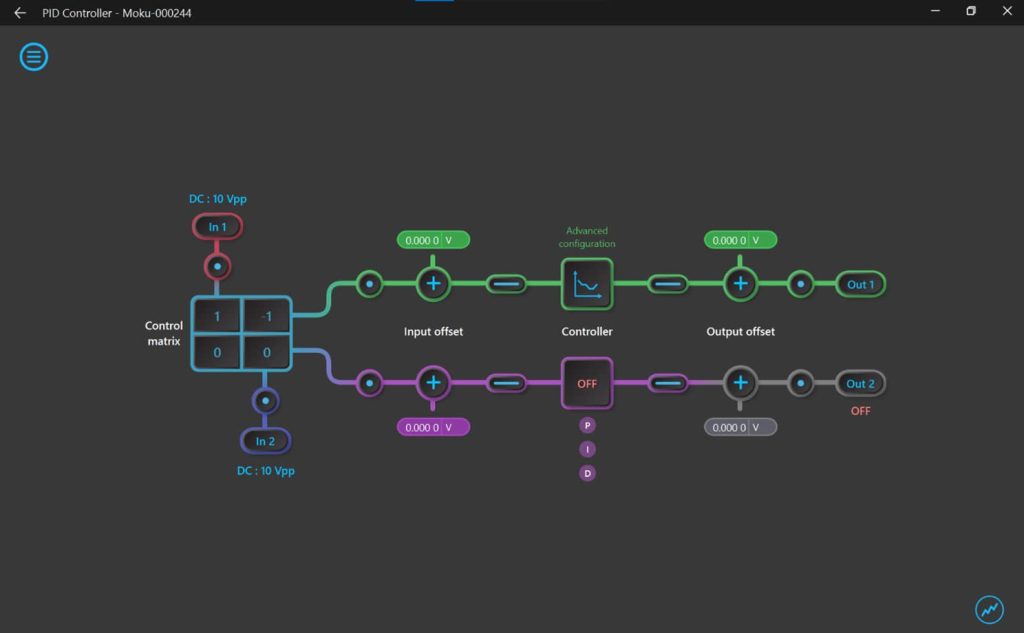
Figure 7: Moku:Go PID Controller
This will open the controller’s parameter settings where you can enter the gains that were just calculated. There is the option to enter the gains in either the frequency-domain or time-domain. The default is the frequency-domain but can easily be switched to the time-domain implementation by checking the box for “Advanced mode” in the bottom right of the controller pop-up window. This mode also allows piece-wise implementation of the controller denoted as Section A and Section B. We will only be using Section A, but you’ll still need to enable Section B and simply disable all parameters except for G (the overall gain) which can be set to 0dB. Remember to enable the correct parameters in Section A by clicking on the P, I, and D symbols on the right.

Figure 8: PID Controller Parameter Settings
Moku:Go’s PID Controller can also be used in real-time to further tune the controller gains and optimize the system response. The PID Controller has an embedded Oscilloscope where signals can be viewed alongside the controller’s Bode plot. By manually changing the gains using the drag and drop method in the Bode plot, students can more readily connect how changing certain gain parameters physically impacts the system. The drag and drop method is only available in the frequency-domain implementation, so being able to convert the PID gains between time-domain and frequency-domain is necessary.
An easy way to view these signals in the embedded Oscilloscope is by clicking on one of the “Probe Points” denoted by a small blue circle enclosed in a larger black circle. They are conveniently placed at points of interest like just after Input 1, just before the PID Controller’s output, and a few other useful places. To view the IR sensor’s output, we would place a probe point after Input 2, marked with a bold A and in red as shown in Figure 9.

Figure 9: PID Controller Probe Points
To confirm that the PID controller actually improves the response of our system, we would now close the loop of our system first connecting Input 1 to the output node of the setpoint potentiometer and then feeding the IR sensor’s output to Input 2 and subtracting it from Input 1 in the control matrix. This simulates the summing block shown in the block diagram of Figure 4. An important step in setting up the closed loop feedback for this lab is to remove the IR sensor’s output offset due to the ball distance. This improves the PID controller response and can be done by adding the offset from the IR sensor when the ball is at rest to the Input Offset in the PID signal path (in this case it is 961.4mV). Then, by applying the same step input used in the open loop part of this experiment by using the setpoint potentiometer, we can capture the closed loop step input response of the system in the embedded Oscilloscope and use the automatic measurements to characterize the response. The closed loop step response of this system can be seen in Figure 10 below which was captured in the embedded Oscilloscope of the PID Controller instrument. This allows us to still run the PID controller and just capture the frame in which the step response is displayed. It is important to use the “Normal” trigger mode so that the signal is captured and displayed correctly for easy measurements.
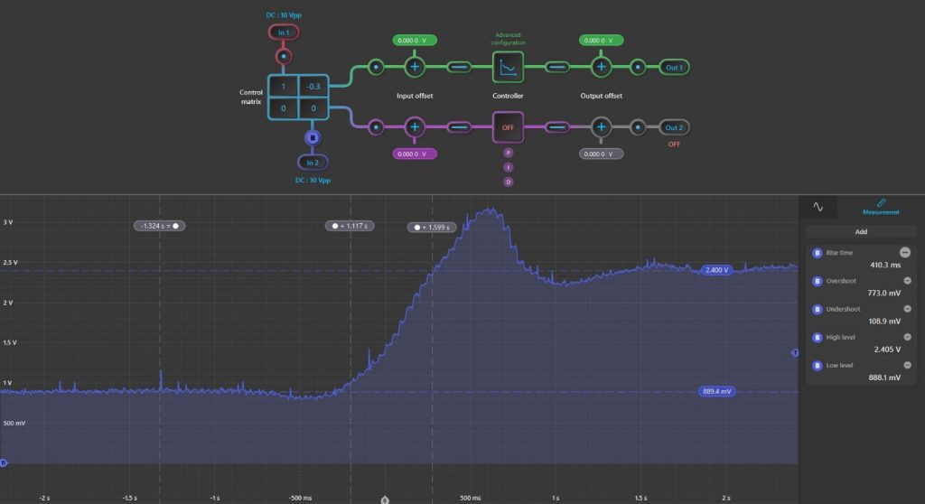
Figure 10: Closed Loop Step Response
Comparing these parameters with the original open loop step input response, we can determine if the PID controller improved the performance of our system. Looking at the automatic measurements from the embedded Oscilloscope, we can see that our time delay, rise time, and undershoot were improved by implementing the PID controller. However, these initial gains also increased our overshoot error significantly. This is expected for the Ziegler-Nichols method we are using and can be easily eliminated by using the heuristics from Table 1 to fine-tune the step response.
The closed loop step response of the tuned system using Table 1 is shown in Figure 11 below.
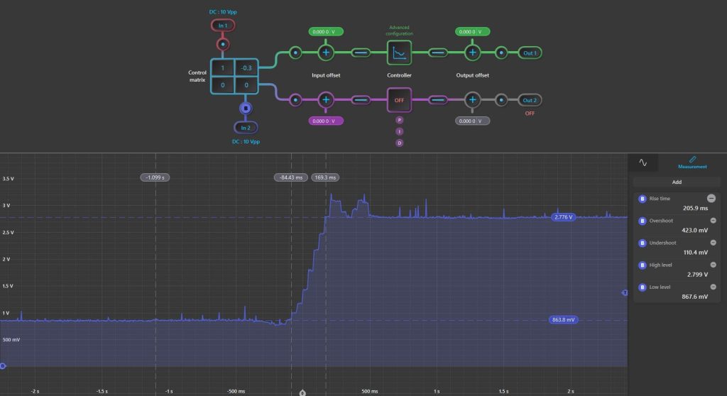
Figure 11: Tuned Closed Loop Step Response
We can see that the rise time, settling time, overshoot, and undershoot are all drastically improved from the open loop response (Figure 6) to the closed loop response (Figure 10) Therefore, we have shown how to visually implement a PID controller lab using common components and the Moku:Go. There were 4 different instruments used within the Moku:Go for this lab including: Oscilloscope, Waveform Generator, PID Controller, and three Programmable Power Supplies (16V and two 5V).

Figure 12: PID Controller Lab Setup
Benefits of Moku:Go
For the educator & lab assistants
- Efficient use of lab space and time
- Ease of consistent instrument configuration
- Focus on the electronics not the instrument setup
- Maximize lab teaching assistant time
- Individual labs, individual learning
- Simplified evaluation and grading via screenshots
For the student
- Individual labs at their own pace enhance the understanding and retention
- Portable, choose pace, place and time for lab work be it home, on campus lab or even collaborate remotely
- Familiar Windows or macOS laptop environment, yet with professional grade instruments
Moku:Go Demo mode
You can download the Moku:go app for macOS and Windows at the Liquid Instruments website. The demo mode operates without need for any hardware and provides a great overview of using Moku:Go.
Have questions or want a printable version?
Please contact us at support@liquidinstruments.com