


Moku:Go

Moku:Go combines 15+ lab instruments in one high-performance device. This application note uses the Moku:Go PID Controller, Oscilloscope, and Programmable Power Supplies to provide a visually engaging way of learning various tuning methods for PID controllers.

Introduction
The Proportional-Integral-Derivative (PID) controller is one of the most common forms of feedback control, and is used in a wide variety of applications like the cruise control in your car or motor control in a drone. The purpose of a PID controller is to drive a process to reach a specified output, typically called a setpoint. The feedback of the controller is used to regulate and optimize the control of this process. Moku:Go features a digitally-controlled PID Controller. The graphical user interface dynamically visualizes the gain profiles, giving the user the ability to drag and drop gain values directly onto a frequency response graph which calculates and displays the transfer function of the PID controller in real time. This allows the student to directly see the poles and zeros of the system as they vary the PID gain values and crossover frequencies.
The purpose of this application is to demonstrate how control theory labs can be updated to better suit the needs of modern undergraduate labs. Typically, control theory is taught through rigorous mathematical modeling with few, if any, physical labs that utilize equipment. This application introduces a modern approach to control theory education by applying a more visual component that helps students more readily connect the theory learned in the classroom to real-life control systems. This is done by controlling the height of a ping-pong ball by using a DC motor fan, an IR distance sensor, and several of the integrated instruments available for Moku:Go. Moku:Go offers 15+ lab instruments, three of which are used for this experiment: the Oscilloscope, PID Controller, and Programmable Power Supplies. Most of these instruments are used simultaneously and can drive the motor control circuitry, take in sensor data, and output a specified signal to control the DC motor’s speed simultaneously. This way, characteristics like the rise time, overshoot, and steady-state height of the ping-pong ball can be controlled and measured from a universal graphical user interface, enabling students to grasp multiple advanced concepts quickly. It also allows real-time tuning through the Moku: app so that students can see how the different PID gains impact the system both mathematically and physically.
Theory of Operation
One Moku:Go will be used in this experiment to power the PCB, read sensor data, implement a PID controller, and generate a control signal. The Moku:Go M2 model has a four-channel programmable power supply unit (PPSU) that is very useful in projects like this and allows it to be a one-box solution for many labs. Two PPSU channels are used in this experiment to power the PCB and the DC fan which is the primary system to be controlled. Moku:Go also has two input channels for reading data and two output channels for generating waveforms. In this experiment, both input channels and one output channel are being used for reading data and generating a control signal. See the figure below for how the PID Demo kit and Moku:Go operate together in a closed-loop system.
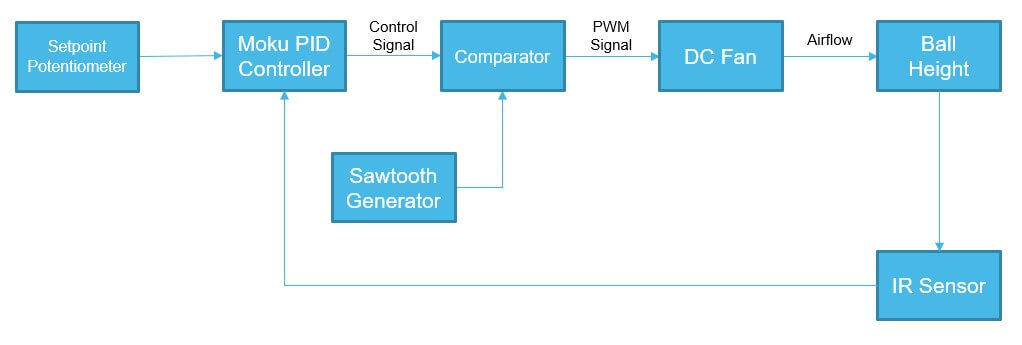
Figure 1: PID demo kit block diagram
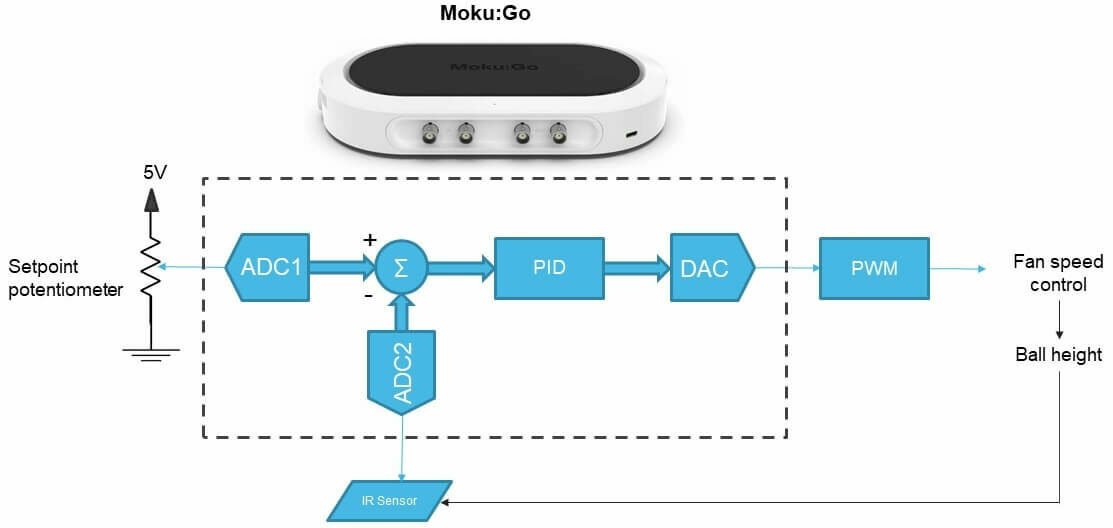
Figure 2: Moku:Go PID controller with demo kit block diagram
ADC1 will read the setpoint signal which is controlled by a potentiometer. ADC2 will read the IR sensor which is affixed to the top of the tube. These two signals are sent to the PID controller running on Moku:Go while the control signal is generated by the DAC and sent to the PWM driver circuit. This control signal will determine the PWM’s duty cycle, which will directly alter the DC fan and, subsequently, the ball’s height inside the tube.
The PWM driver operates by using the NE555 timer (U1) to generate a sawtooth waveform which is fed into the inverting input of the comparator (U2). The PID controller’s output from the Moku:Go (Out1 or DAC1) is fed into the non-inverting input of the comparator, which generates a PWM signal. This signal is sent to a MOSFET (Q2) that controls the power consumed by the 5 V fan. The amount of power the fan sees directly translates to the height that the ping-pong ball will levitate.
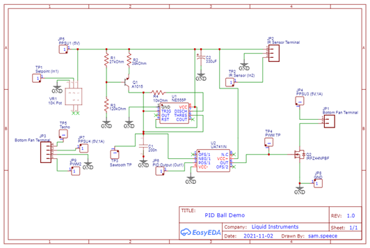
Figure 3: PID controller demo schematic
The other part of this lab setup is the mechanical system used to levitate the ball. It consists of a 5 V DC fan, 3D printed parts (tube, fan connector, and sensor connector), an IR sensor, and a ping-pong ball. The tube has a ¼ inch width slit in the side that acts as variable resistance to the system. There are smaller perpendicular slits marking every 20 mm. The markings should be used to measure from the top of the ball, because this is what the IR sensor sees first. This is important for tuning the PID controller later.
Experimental Setup
Components List
- Moku:Go
- PID Controller Demo PCB
- PID Controller Demo 3D printed parts
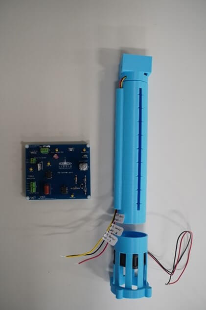
Figure 4: PID controller demo kit
Tuning the PID Controller
Moku:Go PID Controller Setup
The setup for this demo on the PCB can be seen in Figure 5 below. The cables required are two oscilloscope probes, one BNC-to-alligator cable (or BNC-to-mini), and three banana-to-alligator cables. All of these cables (excluding the BNC-to-alligator) are included with Moku:Go.
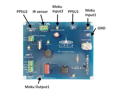
Figure 5: PCB cable setup
Setting up the software for the PID controller is very straightforward thanks to the block diagram style interface that allows students to seamlessly apply control systems theory to real-world practice. Once connected to Moku:Go, open the PID Controller instrument. Set the first row of the control matrix to [1 -0.2]. The control matrix allows for feedback from the physical system by enabling data from Input 2 to be scaled and subtracted from Input 1 (Setpoint). This is very similar to the summation block used in Figure 1. The reason -0.2 is chosen as the scalar is because the dynamic range of the IR sensor must match the dynamic range of the sawtooth generator. Next, set the input offset to -1 V and the output offset to 2 V. The reason for the input offset is because the IR sensor has about a 1 V offset for this system due to the starting position of the ball (about 200 mm away from the IR sensor). The output offset is set to 2 V because the offset of the sawtooth generator is 2 V. Note that you may need to change the input offset based on the average offset of your IR sensor; however, 1 V is a fair starting point.
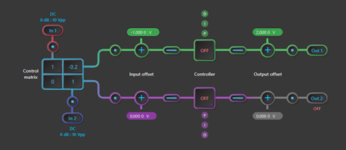
Figure 6: Closed-loop controller setup
The PID controller demo hardware and Moku:Go PID software are now set up for closed-loop tuning.
Open-loop response
Before jumping into the closed-loop tuning method, it may be a good idea to test the system and get an understanding of how it operates and how to control it. The open-loop response of a system is a very common and straightforward measurement to make that involves sending a step input to the system under test and measuring its response. This can be done by setting the PID Controller’s control matrix to [1 0], the input and output offsets to 0 V, and enabling the proportional gain to 0 dB. This setup allows the output to track the input, which is the voltage being read by Input 1 from the setpoint potentiometer.
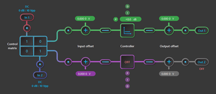
Figure 7: Open-loop controller setup
Vary the setpoint potentiometer and you’ll notice the ball height change. To view the setpoint potentiometer signal, enable a probe point after Input 1 (click the red probe point icon) and enable a tracking cursor to more readily see the setpoint voltage as the potentiometer is varied.
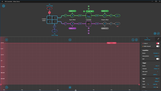
Figure 8: Setpoint potentiometer signal
To take the open-loop step response measurement, enable a probe point at Input 2 (IR sensor), set the trigger mode to Normal, and the trigger channel to Probe B. Choose a suitable height for the ball using the setpoint potentiometer and then disable the output by clicking Out 1. By choosing a suitable trigger level based on the ball height chosen, once the controller output is enabled again the ball will rise to its previous position and resemble a graph like the one in Figure 9 below.
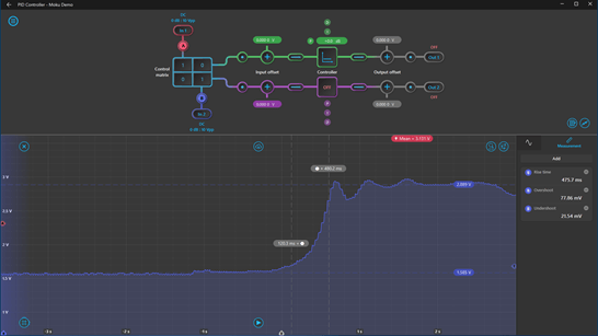
Figure 9: Open-loop step response
The embedded oscilloscope also has cursors and automatic measurements that allow quick characterization of the open loop response signal.
Closed-loop PID Controller tuning
There are a couple of well-known manual tuning methods for PID controllers, one of which is known as the Ziegler-Nichols method that uses the open loop response of the system to determine the PID gains, and is done in another application note found here. This application will use a closed loop method that gives reasonably stable results. Before starting the closed loop tuning make sure to reset the controller settings to resemble those of Figure 6.
a. Open the PID Controller instrument, turn on only the proportional gain and set it to 0 dB. Adjust the setpoint potentiometer until the ball is at the desired height for tuning. The PID controller parameters will have different values than those below if the starting height is different. This application starts the ball at 60 mm, or Vsetpoint = 2.1 V (60 mm to the top of the ball since this is what the IR sensor sees).
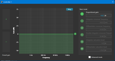
Figure 10: Proportional gain setting
b. Increase the proportional gain until the ball starts to oscillate. Remember that you can use the mouse to drag the gain and adjust it directly on the graph. There is also the option to use the mouse wheel to scroll over the numbers to adjust it, or type in the value manually.
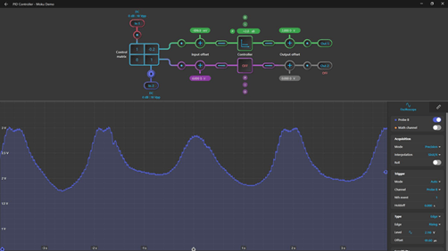
Figure 11: System oscillation graph
c. Enable the differentiator gain to its highest crossover frequency and decrease the differentiator crossover frequency until the oscillations stop (or are greatly reduced as the ball will usually have some small movement in the tube due to the sensor noise).
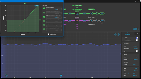
Figure 12: PD controller values and system response
d. Enable the integrator gain at its lowest crossover frequency. This will cause the controller to saturate, so enable the integrator saturation level as well. This will limit the integrator crossover frequency so the system does not saturate either. The ball will have increased in height after enabling these two parameters so before tuning any further, decrease the proportional gain until the ball is at the same height as when the tuning was started in step a (in this case around 60 mm).
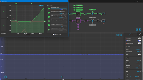
Figure 13: PID controller values and system response
If the ball starts oscillating at a magnitude similar to step b then adjust the integrator crossover frequency and differentiator crossover frequency until the IR sensor output is similar to Figure 13 above.
e. Now that the initial PID gains have been found, further tuning of the system can be done by trial-and-error using the table below as a guide for adjusting each gain based on the closed loop response to a step input. It is important to vary the setpoint between the minimum and maximum points while tuning for optimal gain values.
Table 1: PID gains tuning guide
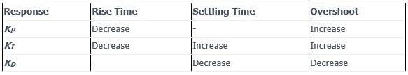
Keep in mind that when increasing KP, the setpoint will need to be decreased to maintain the same ball height. Feel free to drag the P, I, or D gain values around directly on the transfer function graph to see how each gain value changes different aspects of the system. Do the assumptions in the table above match how the system responds to changes of the associated gain values in the PID controller?
f. Use the built-in oscilloscope within the PID Controller to obtain measurements for characterizing the system by placing a probe point inside the PID controller signal chain. The IR sensor feedback should be on Input 2. There is also a digital switch before and after the PID controller block which is helpful for stimulating the system with a step input without the need for a physical switch or unplugging cables constantly.
Below is a well-tuned response for a step increase to the desired 60 mm ball height.
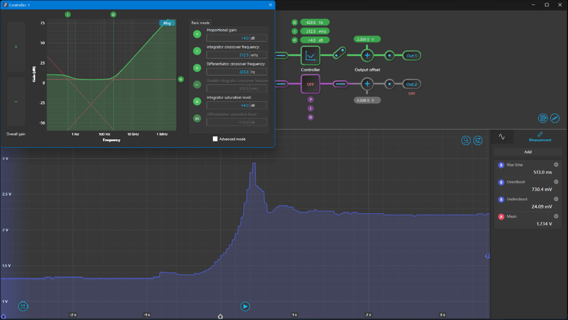
Figure 14: Tuned PID controller gains and system response
This step response is from the low level 40 mm input to the high level 160 mm input using the setpoint potentiometer. It is interesting to note the still relatively high overshoot of the graph despite the ball barely going above the desired setpoint. This can be explained by the IR sensor’s datasheet where there is a non-linearity in the sensor output voltage as an object gets within 40 – 50 mm of the sensor which results in a seemingly large overshoot in our system.
Conclusion
This application note showed how to tune a closed-loop control system using the Moku:Go PID Controller to improve common system characteristics like rise time, overshoot, and steady-state error. Alongside the PID Controller, this note also used the integrated Oscilloscope, Waveform Generator, and Programmable Power Supplies that powered and controlled the circuit drivers and DC fan. The visualization of how a PID controller functions by use of a floating ping-pong ball alongside the interactive transfer function graph benefits students and professors looking to add depth to their control theory course through a hands-on, highly visual example. The Moku:Go PID Controller can help students connect theory to real-world implementation through this experiment.
Benefits of Moku:Go
For the educator & lab assistants
Efficient use of lab space and time
Ease of consistent instrument configuration
Focus on the electronics not the instrument setup
Maximize lab teaching assistant time
Individual labs, individual learning
Simplified evaluation and grading via screenshots
For the student
Individual labs at their own pace enhance the understanding and retention
Portable, choose pace, place and time for lab work be it home, on campus lab or even collaborate remotely
Familiar Windows or macOS laptop environment, yet with professional grade instruments
Moku:Go Demo mode
You can download the Moku:Go app for macOS and Windows at the Liquid Instruments website. The demo mode operates without need for any hardware and provides a great overview of using Moku:Go.
Acknowledgements
We would like to thank Dr. Vivek Telang for his time and help in designing this project to be used for further Control Systems education. If you would like to get in touch with Dr. Telang for questions regarding this application note, please contact him at vivek.telang@utexas.edu.