Reducing noise and transients with custom real-time digital filtering

Moku Cloud Compile

Moku Cloud Compile (MCC) is a Liquid Instruments service that allows you to quickly compile and deploy custom hardware description language (HDL) code to a Moku device. MCC opens the FPGA within the Moku to custom code and allows users to develop specific functions and features. We provide a range of examples and support to help you to deploy custom functions.

 

Moving average filter

A moving average filter is quite simply an average of a number (n) of consecutive signal samples. The equation is:

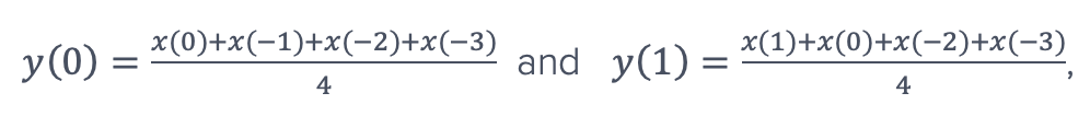
Where x(t) is the discrete time series input signal and y(t) is the output signal. For example, when n = 4:

This simple filter has a very useful application in the reduction of noise in a signal. For uncorrelated, random (white) noise, this moving average function is optimal for rejecting the noise and retaining a sharp step response, while having poor stopband performance. Implementing this in hardware requires only adders and one division and is thus useful with limited hardware resources. Division by an arbitrary number in hardware is not simple in an FPGA. Typically, this filter is implemented by ensuring n is a power of 2 (i.e., n = 2^N), reducing the division to a right shift of N binary bits.

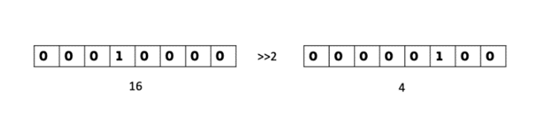
Figure 1: Binary bitwise shift

A direct hardware implementation would look like Figure 2.

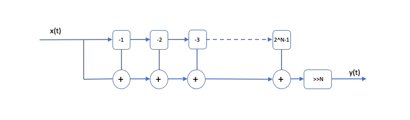
Figure 2: Series of adders to implement a moving average

This implementation would require 2^N-1 adders and is expensive in terms of hardware. The deep series of adders would also likely require clocked registers to meet reasonable timing performance. We can improve upon this by realizing:

Thus, more generally illustrated in Figure 3:

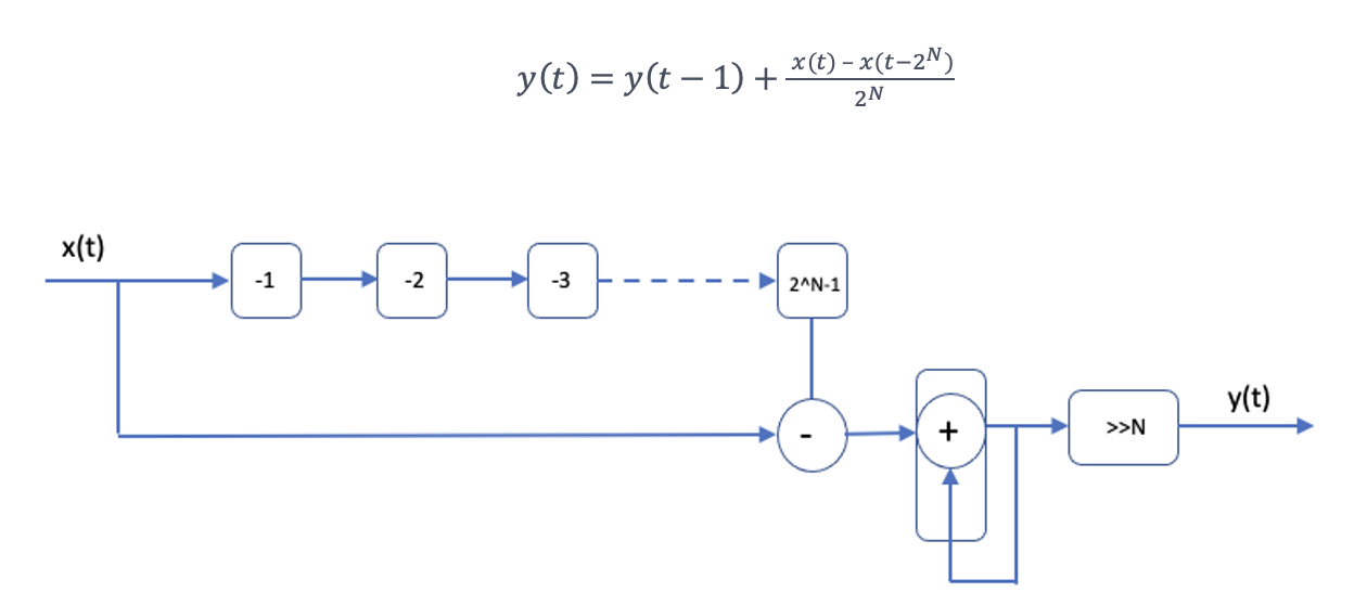
Figure 3: Accumulator implementation

This recognizes that each output depends upon the prior output and the current input. We have now reduced the moving average function to an accumulator, one subtraction function, and an n-stage shift register followed by a bitwise right shift for the 2^N division (Figure 3). When N > 4, this hardware saving becomes significant, and the limiting factor is the 2^N stage shifter register. Additionally, no further clocked elements are needed to meet timing constraints.

 

VHDL implementation

Figure 4 shows the core of the VHDL implementation. The core of this filter is very simple and has just 12 lines of code. The p_moving_average is the time history of the last N samples, where line 8 is prepending the newest input and dropping the oldest. On line 9, the accumulator r_acc is adding the new input, while line 10 is generating the bitwise shift (divider) needed for the output.

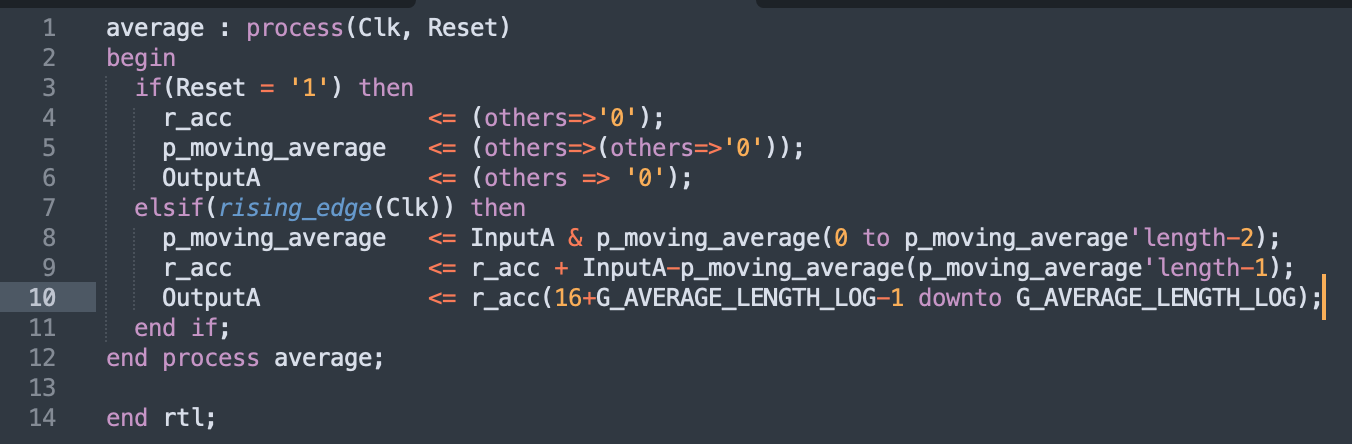
Figure 4: Moving average VHDL code

Compile and deploy

It’s easy to compile and synthesize this VHDL code. To get started, visit compile.liquidinstruments.com, upload the code, and select build. The Liquid Instruments server will produce a file or bitstream that defines the hardware configuration needed on the FPGA to implement the code. For Moku:Go and Moku:Lab, compilation takes approximately 5 minutes; for Moku:Pro, it’s closer to 20 minutes due to the much larger size of the FPGA.

Detailed instructions to guide you through the compilation and deployment are available here.

 

Testing the MCC moving average filter

To test this moving average filter, we use Multi-instrument Mode (MiM) for Moku:Go as shown in Figure 5. In this mode, we can deploy two instruments with a sample rate of 31.25 MHz. We could also test this filter on Moku:Pro, which allows for four simultaneous instruments in MiM and an input sample rate of 312.5 MHz.

 

Slot 1 contains our Moku Cloud Compile moving average filter, while Slot 2 contains the Oscilloscope instrument. We use the Oscilloscope to observe the filtered and unfiltered signals fed from analog-to-digital (ADC) Input 1. The Oscilloscope also has an integrated Waveform Generator, used to generate the test signals. In this case, we generate a square wave using the Oscilloscope’s built-in Waveform Generator at 2 kHz and drive it to Output 1. We attenuate the signal by 60 dB externally, driving it close to the noise floor of Moku:Go. We then route this signal back into Input 1.

 

 

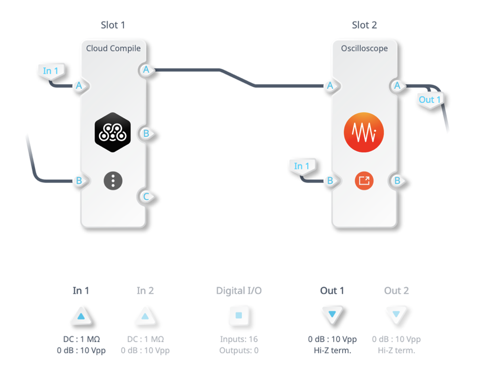
Figure 5: Filter test setup in Multi-instrument Mode

In Figure 6, we can see the noisy square wave after attenuation in the blue trace. The red trace shows the moving averager’s output with a significantly cleaner square wave. This is a useful noise reduction technique that has been enabled using one slot of MCC and MiM.

Figure 6: Noise reduction using the MCC moving average filter

This simplest of filters has thus been useful in reducing noise. It is also very computationally light, requiring only an accumulator, subtractor, and bit-wise shift. This means it can run at very high speeds of 312.5 MSa/s on Moku:Pro or 31.25 MSa/s on Moku:Go.

Turning our attention to the noise power, we know that this average filter reduces the noise power by a factor of 2^N; the noise amplitude is reduced by √2^N. Our implementation uses N=8, so noise amplitude should be reduced to 6.25% (1/16) of the original.

Figure 7 shows the Moku:Go input noise (blue trace) and the moving average signal (red trace) with amplitudes of 161.2 mV and 9.162 mV, respectively. From this, we can see that the amplitude of the noise after the filter is close to the expected factor of 1/16 the original noise, or 9.162 / 161.2 mV = 0.057. This filter is operating and meets our expectations.

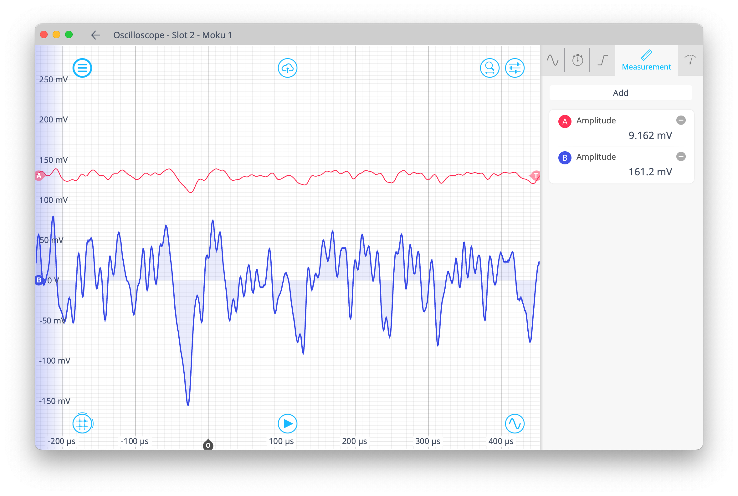
Figure 7: Averaged input noise

Frequency response

We can readily determine the frequency response of the moving average using the Moku Frequency Response Analyzer (FRA) instrument. The FRA drives a frequency-swept sine wave on its output and measures the resulting amplitude and phase on its input. Figure 8 shows the test setup:

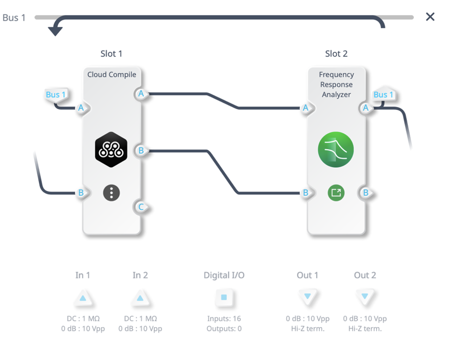
Figure 8: Frequency Response Analyzer MiM configuration

Figure 9 shows the resulting frequency response of the MCC filter. Comparing this with Figure 10, a MATLAB plot of an ideal moving average filter, we see that the moving average filter does not provide a particularly good stopband attenuation.

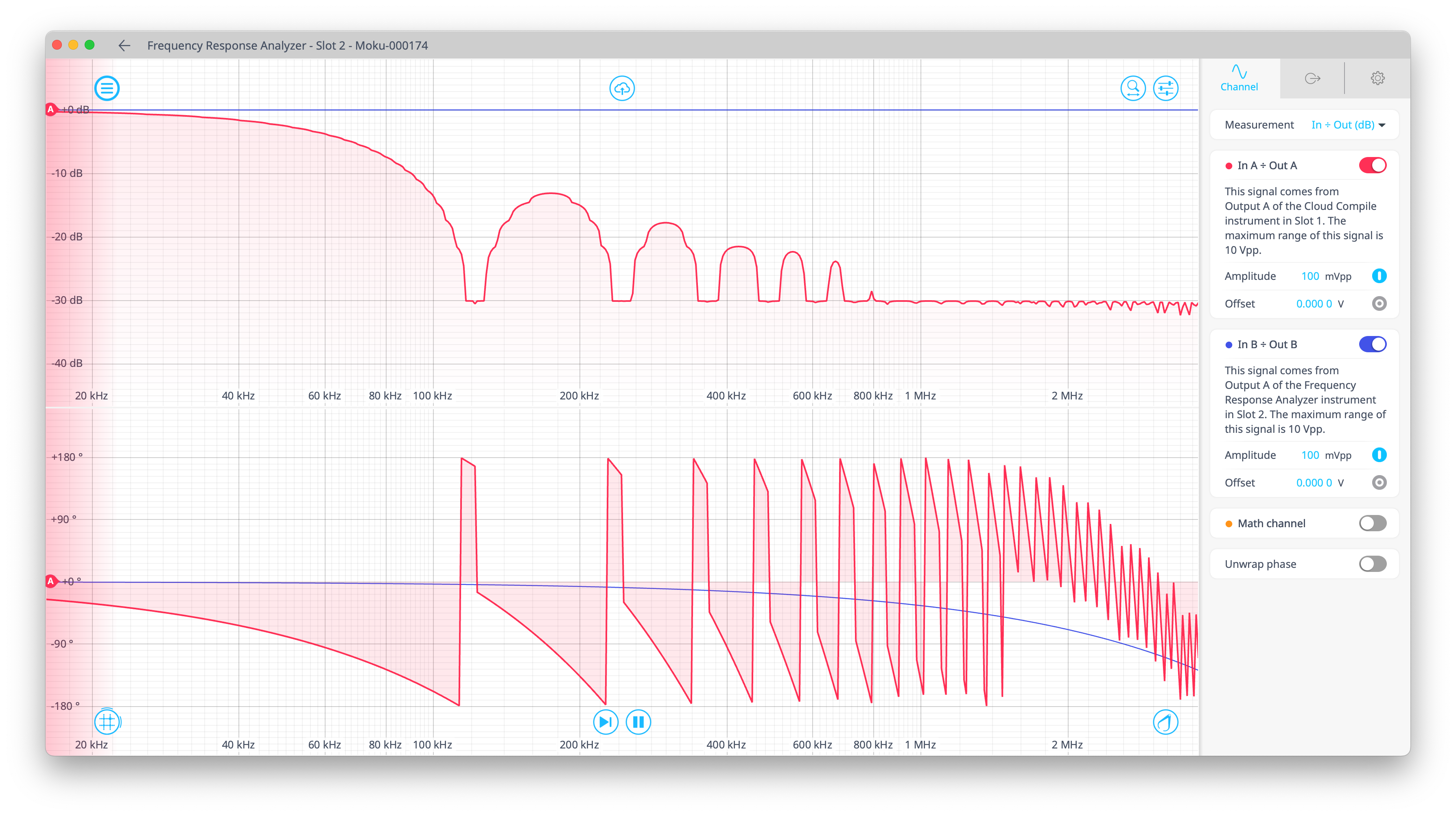
Figure 9: Frequency response of the moving average filter

                                                                                       

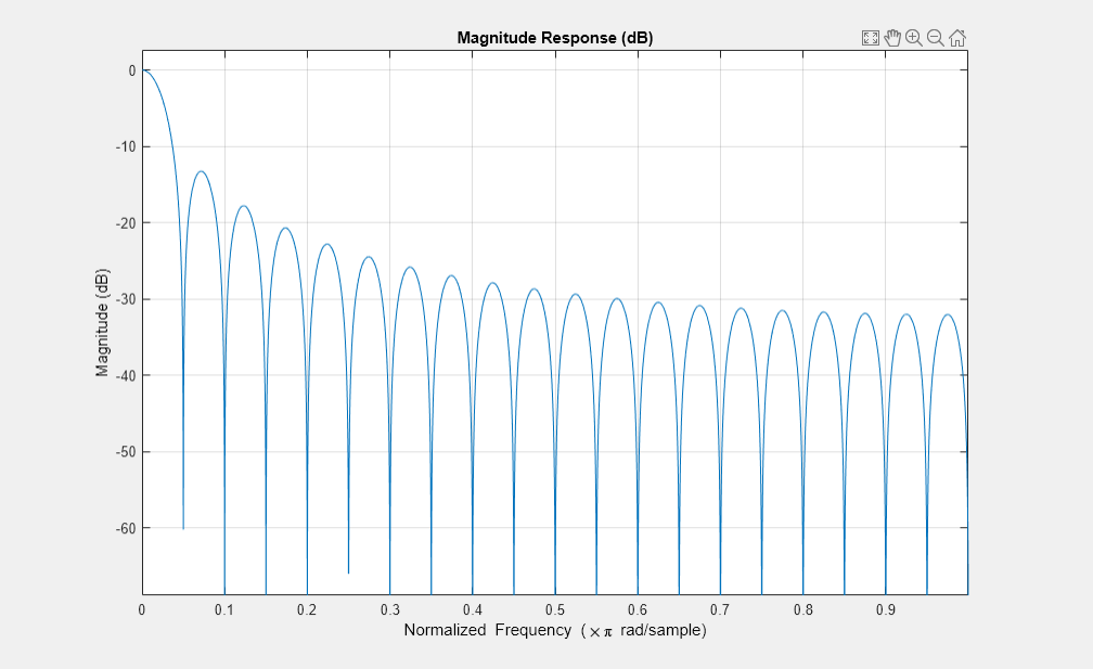
Figure 10: MATLAB plot of ideal moving average filter

Median filter

A median filter is a nonlinear filter that determines the median value of a small moving window. The input samples pass through the window and the output is the median of the samples at any given time. While a moving average filter is good for filtering evenly distributed random noise, a median filter is appropriate for filtering out very short spikes or impulse noise. While it is often deployed in image processing, it is also useful in more general signal processing.

Typically, an odd number of samples is chosen for the window length: 3, 5, or 7 points. This means that the output is simply the middle sample of the value-ordered window.

 

VHDL implementation

Figure 11 shows the implementation of a five-point median function in VHDL. At each rising edge of the clock signal, the function in Figure 11 sorts the five input samples from low to high values. This sorting occurs in the two nested “for” loops from lines 12 to 20. Thus, the median is the third sample in the sorted window; this is assigned to the output on line 22.

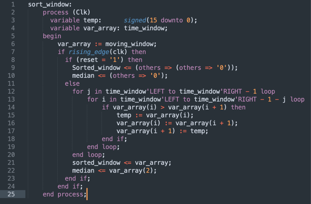
Figure 11: Median filter VHDL code

We can analyze the time-domain performance of the median filter in the same manner as the moving average filter by using the Oscilloscope and Moku Cloud Compile slots with the Waveform Generator of the Oscilloscope.

Figure 12 shows significantly reduced noise peaks, lowering the peak-to-peak measurement of unfiltered noise from 3.66 mV to 305 μV after filtering. This is a reduction of 1/12, which is not as effective as the moving average filter (1/16).

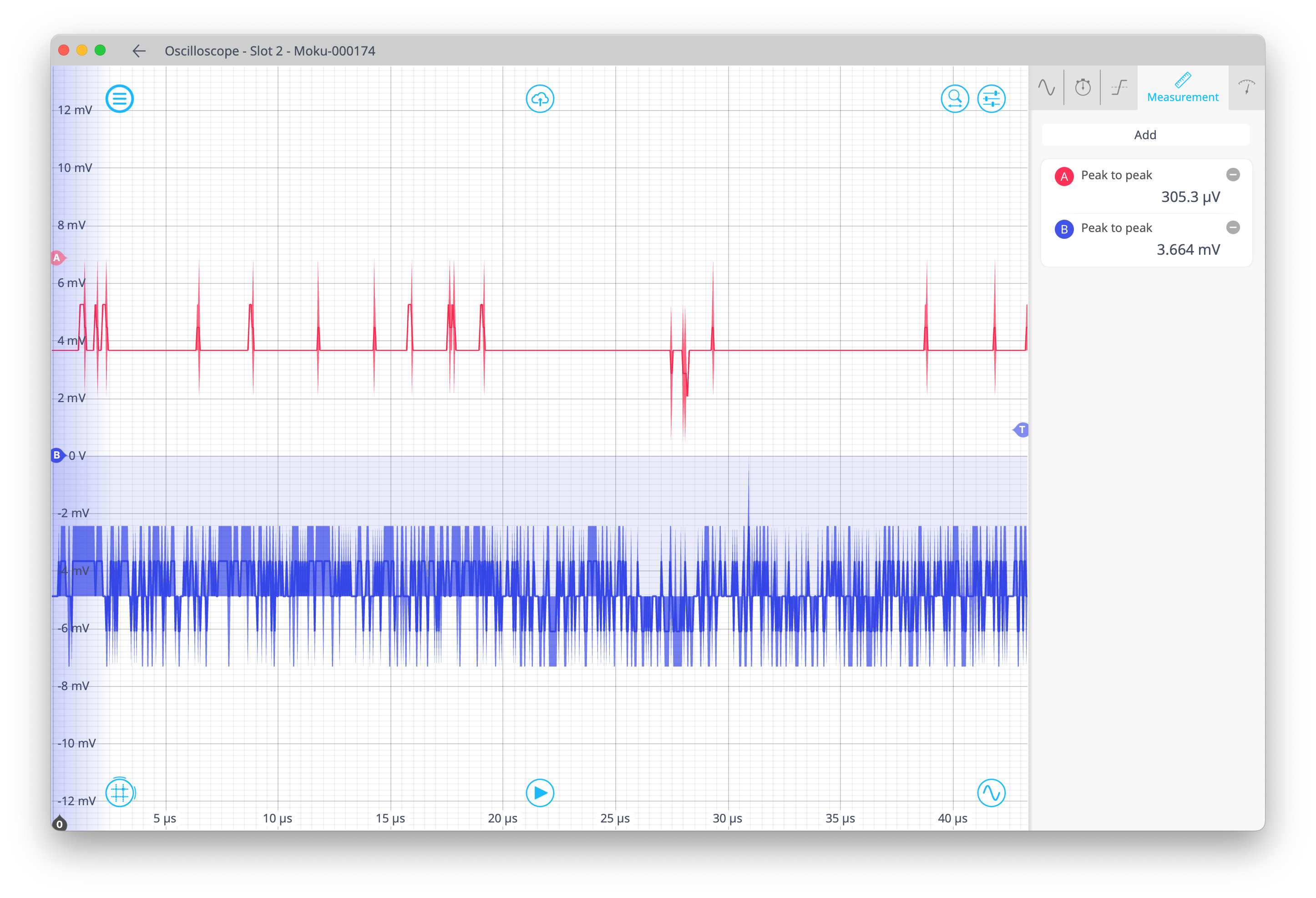
Figure 12: Median filter time-domain performance

Since a key function of the median filter is to remove impulse noise, we also examine its performance with a square wave with added impulses. Figure 13 shows a square wave with a leading-edge spike and a spike halfway through the low level (blue channel B); the filtered signal shows the square wave after the median filter has removed the spikes but retained the sharp lead and trailing edges (red channel A).

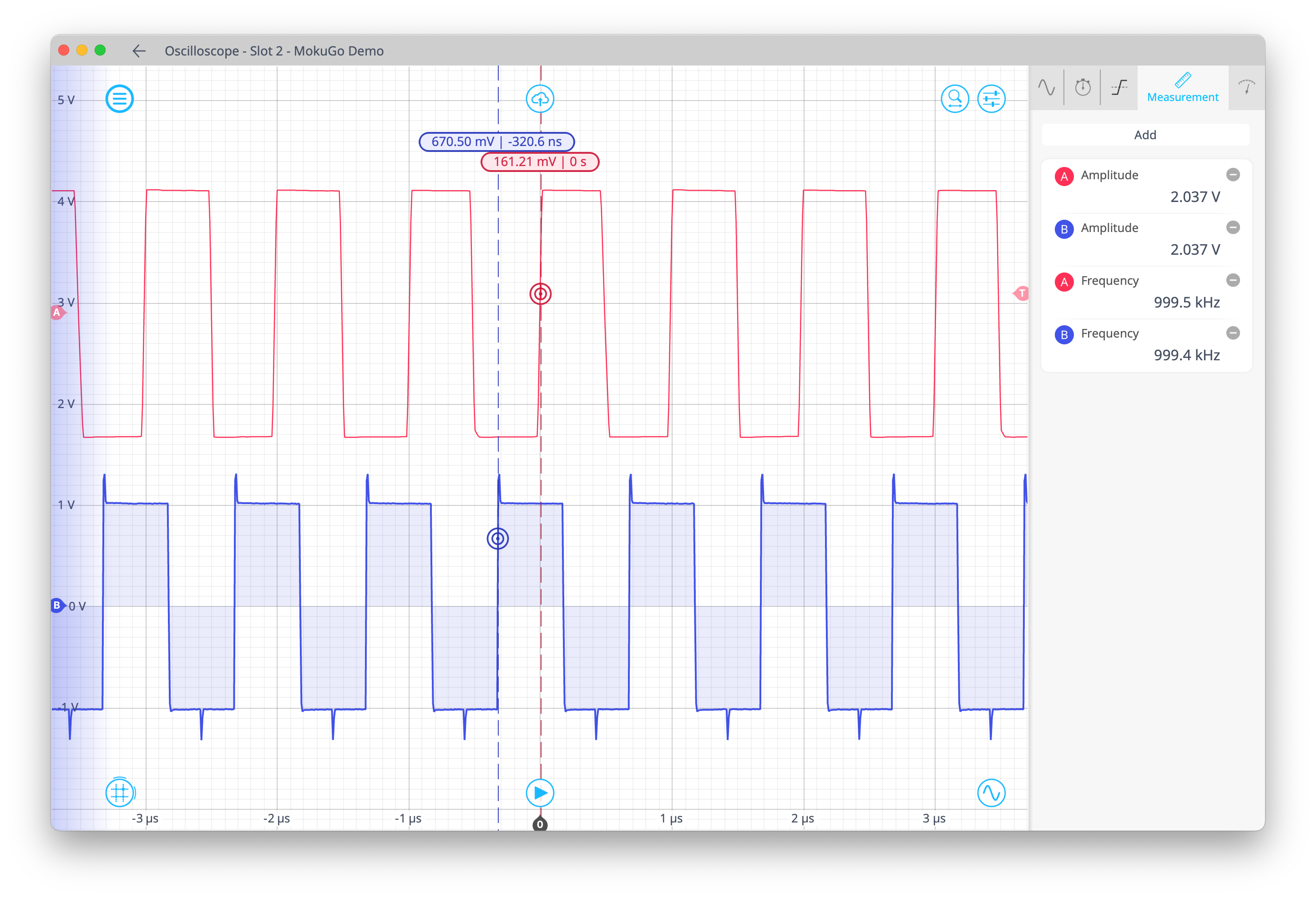
Figure 13: Median removing spike noise

We compiled and tested this median filter on Moku:Go, which has an MCC clock rate of 31.25 MHz. However, when testing this example for Moku:Pro, we needed to adjust our implementation due to an increased clock rate of 312.5 MHz. The implementation in Figure 11 uses a nested-for loop with variables. This synthesizes to a large and deep combinatorial logic net with a propagation delay (Figure 14) that exceeds the 3.2 ns period of the Moku:Pro clock rate. To meet timing, the propagation delay of the logic between clocked elements must be less than the clock period.

Figure 14: Propagation delay through logic

We need to break the large logic block into segments separated by registers or clocked elements. In VHDL, we achieve this by using signals as opposed to variables. In this case, we break the logic into five stages for ease of coding. This means that there is an input-to-output latency of around five clock cycles, which is suitable for our application.

Figure 15 shows one stage of this five-stage pipelined median algorithm. Find the full VHDL in the project files available for download here.

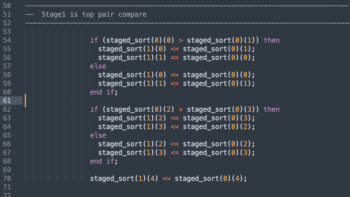
Figure 15: One stage of pipelined median filter

Moku:Pro median filter testing

We use Moku:Pro in MiM with an Arbitrary Waveform Generator (AWG) to create a square wave with noise spikes. We then connect the output of the AWG to the MCC median filter and observe the effects with an Oscilloscope.

This MiM setup is shown in Figure 16. We configured the AWG as shown in Figure 17. Its output is driving an analog signal to Output 3 of Moku:Pro, which in turn is looped via a coaxial cable to Input 3. We deployed the median filter in the Moku Cloud Compile slot and used the Oscilloscope to observe the performance.

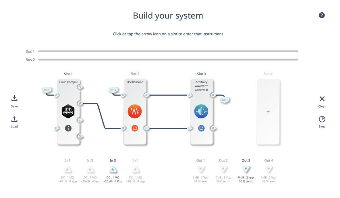
Figure 16: Moku:Pro Median filter test system

Finally, we observe the median filter’s performance, shown in Figure 18. The median filter has removed the impulses while retaining the sharp edges of the square wave. The processing delay caused by the insertion of the staged, clocked pipeline leads to approximately 44 ns latency.

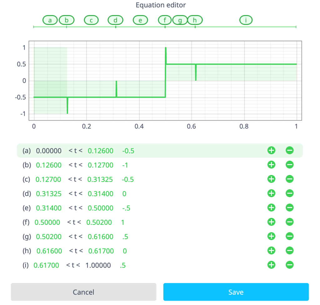
Figure 17: Arbitrary Waveform Generator, square wave with impulses

 

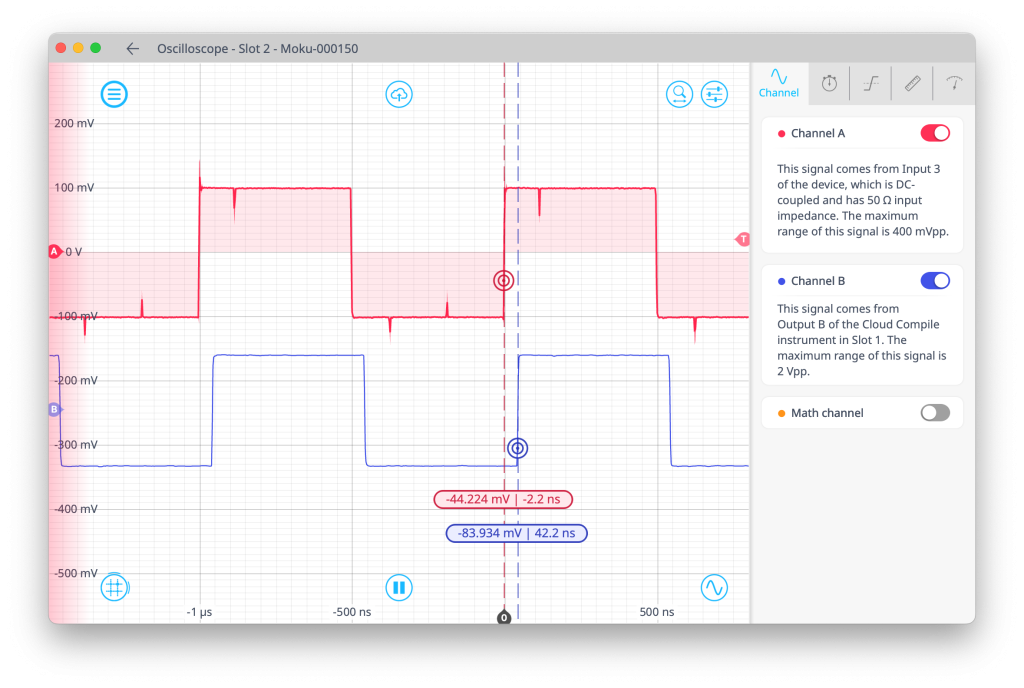
Figure 18: Moku:Pro median filter operation

Summary

In this application note, we discussed the implementation of a moving average filter and a median filter. To implement these, we utilized Moku Cloud Compile to build our filters and deployed them to a Moku:Go device. We then modified our design to ensure compatibility with the increased Moku:Pro clock rate. To validate the MCC filter behaviors, we used Multi-instrument Mode to connect the fully customizable filters, an Oscilloscope, and an Arbitrary Waveform Generator. This implementation enables efficient noise reduction while preserving signal edges in digital signal processing applications.

Code download

The code for the application note is available for download here.

Moku: demo mode

You can download the Moku: app for macOS and Windows on our website. The demo mode operates without any hardware and provides an introduction to using either Moku:Go, Moku:Lab, or Moku:Pro. The Moku: app is also available for iPadOS in the Apple App Store.

Questions or want a printable version?

Contact us at support@liquidinstruments.com.

Reference

[1] www.mathworks.com/help/dsp/ug/how-is-moving-average-filter-different-from-an-fir-filter.html