Updated October 1st, 2025
The Moku Phasemeter measures phase with up to 6 µradian precision for input signals oscillating between 1 kHz and 2 GHz. Using a digitally implemented phase-locked loop architecture, it provides exceptional dynamic range and precision far exceeding the capabilities of conventional lock-in amplifiers and frequency counters. The Phasemeter calculates and plots Allan deviation, which is a unitless measure of stability, typically used to quantify the stability of clocks and other oscillators. In this guide, we will cover the math and provide an example Allan deviation calculation with the overlapped variable \(\tau\) estimator.
To learn more about Allan deviation and phase measurements, watch our webinar on quantifying modern clocks and oscillators.
To download this application note, click here.
Allan Deviation with overlapped variable τ estimators
Allan deviation is measure of stability, typically used to quantify the stability of clocks and other oscillators. The Allan deviation \(\sigma_y\) of the frequency \(y\) is calculated as a function of observation time \(\tau\) by the following equation:
\(\sigma^2_y(\tau) = \frac{1}{2}\langle \left( \bar{y}_{n+1} – \bar{y}_n \right) \rangle\)
Alternatively, the phase measurement, \(x\), can be used to measure the Allan deviation. The phase and frequency relate as phase is the integral of the frequency \(x = \int{y \ dt}\), and the expression becomes:
\(\sigma^2_y(\tau) = \frac{1}{2\tau^2}\langle \left( x_{n+2} – 2x_{n+1} + x_n\right) \rangle \)
where \(x\) is the phase measured over time. In practice, it’s not possible to calculate the expected value over infinite time. When using hardware with a finite sampling rate and time, we must discretize this equation. The Moku Phasemeter uses the overlapped variable \(\tau\) method to calculate the Allan deviation, which is defined as:
\(\sigma^2_y(n\tau_0, N) = \frac{1}{2n^2 t_0^2 (N-2n)} \sum^{N-2n-1}_{i=0}{ \left( x_{i+2n}-2x_{i+n}+x_i \right)^2} \)
where \(\tau_0\) is the sampling period of the Phasemeter and \(N\) is the number of data points acquired for the input time series. \(n\) is an integer multiplier of the sampling period that best estimates the desired \(\tau \simeq n \tau_0\). \(x_i\) represents the ith element in the time series.
Allan Deviation with the Moku Phasemeter
In this example, we measured the Allan deviation of a 1 MHz signal with Moku:Pro Phasemeter. The frequency of the signal was measured at 150 Hz for 10 minutes. To display the Allan deviation, select the “Frequency” tab on the top of the Moku display and “Allan deviation” in the plot area.
Please note that Moku Phasemeter only calculates the Allan deviation of the frequency using phase information as shown above. Selecting the “Phase” or “Amplitude” tabs will not change the Allan deviation plot.
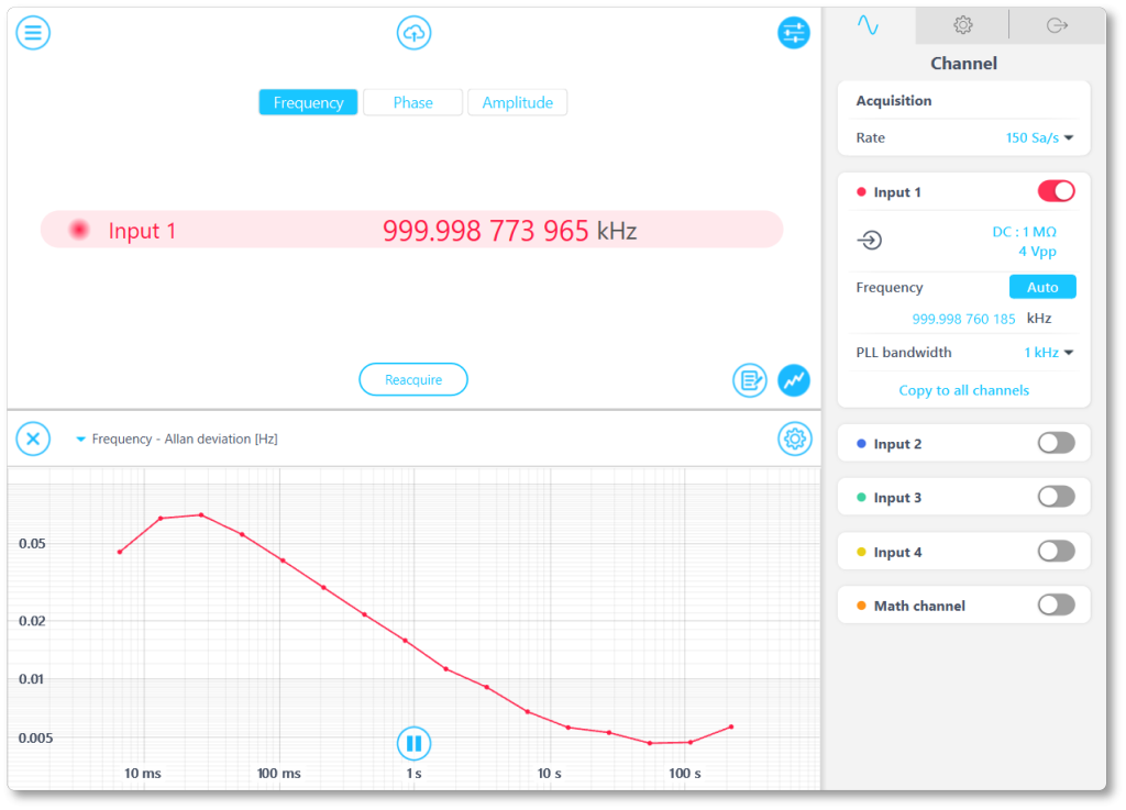
Figure 1: Phasemeter on Moku:Pro displaying Allan deviation of 1 MHz signal.
Python implementation
We will verify the accuracy of the phasemeter by performing the same calculation in Python. The function cal_oadev takes the time series of the phase information, sampling rate and an array of observation time \(\tau\) as the input. It calculates the overlapped Allan Deviation using the above equation and returns \(n\tau_0\) and \(\sigma_y (n \tau_0)\) as arrays.
Using this function requires the NumPy and math libraries.
#Import libraries
import numpy as np
import math

def cal_oadev(data,rate,tauArray):
    tau0 = 1 / rate  # Calculate the sampling period
    dataLength = data.size # Calculate N
    dev = np.array([]) # Create empty array to store the output.
    actualTau = np.array([])

    for i in tauArray:
        n = math.floor(i / tau0) # Calculate n given a tau value.
        if n == 0:
            n = 1 # Use minimal n if tau is less than the sampling period.

        currentSum = 0 # Initialize the sum
        for j in range(0, dataLength - 2*n):
        # Accumulate the sum squared
            currentSum += (data[j+2*n] - 2*data[j+n] + data[j])**2

        # Divide by the normalization coefficient
        devAtThisTau = currentSum / (2*n**2 * tau0**2 * (dataLength - 2*n))
        dev = np.append(dev, np.sqrt(devAtThisTau))
        actualTau = np.append(actualTau, n*tau0)

    return actualTau, dev #Return the actual tau and overlapped Allan deviation
Example calculation
In this example, we imported the time series we acquired previously on the Moku and calculated the Allan Deviation with Python scripts. You can find all the raw data and scripts here.
The time series can be found in the “data.csv” file. This data is obtained by using the embedded Data Logger on the Phasemeter. The first column is the measured time in seconds, and the fourth column is the measured phase in cycles. The script “CalculateAllanDeviation.py” reads the excel file and calls the cal_oadev function in the “AllanFunc.py”. The Allan Deviation is plotted as a function of \(\tau\) in log scales. The Allan Deviation plots matched well between the Moku:Pro and Python scripts.
Running this analysis requires the matplotlib and pandas libraries.
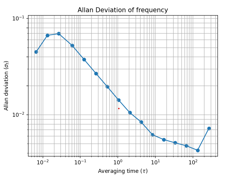
Figure 2: Allan deviation calculated using python on logged phase information.
References
[1] Land, D. V., A. P. Levick, and J. W. Hand. “The use of the Allan deviation for the measurement of the noise and drift performance of microwave radiometers.” Measurement Science and Technology 18, no. 7 (2007): 1917.
[2] Allan, David W. “Statistics of atomic frequency standards.” Proceedings of the IEEE 54.2 (1966): 221-230.
[3] Howe, D.A., Allan, D.W., and Barnes, J.A. “Properties of signal sources and measurement methods.” Proceedings of the 35th Annual Symposium on Frequency Control (1981): TN-14 – TN-60.