Multi-Instrument Mode on Moku:Pro allows you to lock lasers to optical cavities with the Laser Lock Box while also measuring the Bode plots by using the Frequency Response Analyzer with no additional test equipment or wiring. By injecting a disturbance into the error signal and measuring the transfer function using the Frequency Response Analyzer, you can check the closed-loop gain, phase margin, and loop disturbance rejection performance. The flexibility of quickly switching between the Frequency Response Analyzer and Laser Lock Box makes it convenient for you to adjust PID parameters and optimize loop performance to ensure stability and maximize disturbance suppression.
In high-precision measurements, such as molecular and atomic physics applications, laser systems with active frequency noise suppression are widely used, due to their good long-term stability. Achieving a stable laser lock requires a highly optimized feedback controller, which especially involves measuring: 1) the transfer function of the control loop, ensuring that there is sufficient gain at low frequencies while keeping the unity-gain frequency low to maintain loop stability; and 2) disturbance rejection, the response as a function of frequency that a disturbance would experience if it were coupled into the laser and detected after passing through the entire system.
The transfer functions are normally plotted as a Bode plot, representing the gain and phase shift of the loop taken over a set frequency range. The main challenge in measuring the closed-loop disturbance rejection is injecting noise without interrupting the feedback control. Normally, the system setup is very complex, requiring both a noise source as an injection method and a network analyzer to measure the response.
In this application note, we’ll demonstrate how to use Multi-Instrument Mode on Moku:Pro to characterize the open-loop and closed-loop performance of a laser stabilizing system. Moku:Pro enables us to lock the laser to the cavity, inject the disturbance, and simultaneously measure the open-loop, closed-loop, and disturbance transfer functions. You can adjust PID parameters to optimize the loop configuration to ensure stability, enhance disturbance suppression, and suppress frequency noise. Moku:Pro provides a compact and efficient solution for laser stabilization and characterization.
Feedback control basics
To better understand a laser locking system, we must first start with a brief review of generic feedback control. By analyzing and deriving the disturbance rejection equations in this section, we can begin to determine where to inject the disturbance as well as where to probe for a loop response in the Pound-Drever-Hall (PDH) locking procedure.
In general, we can divide control systems into two types, namely, open-loop control systems and closed-loop control systems. The main difference is that the control action of the former is independent of the output of the system, whereas the latter has an output dependent control action [1]. The basic idea of a generic feedback control loop is to maintain the output of a system operating at a constant setpoint by using the difference between the current operating point and a reference as an error signal [1]. The PDH locking technique for laser stabilization utilizes the cavity reflection to generate an error signal, which feeds back to the laser to maintain the optical source lasing at a certain frequency with minimal laser frequency noise. This is considered closed-loop control [2]. An elementary feedback control system normally has three components as illustrated in Figure 1, naming a plant (which is to be controlled), a sensor (which measures the output of the plant), and a controller (which generates the feedback input).

Figure 1: The block diagram of a typical feedback control system. It consists of three major objectives: the plant (P), the sensor (S) measuring certain signals, and the actuator or controller (C) generating the input to the plant.
We can derive the transfer function of a control system using the Laplace transform, which is defined as \(F(s)\) for a given time-domain signal \(f(t)\).
\(F(s) = \int{e^{-st} f(t) dt}\)
For the system shown in Figure 1, each of the three components has its own transfer function, denoted as \(P(s)\), \(S(s)\), and \(C(s)\) for the plant, sensor, and the controller, respectively. To simplify the following derivation, an extra internal signal has been introduced and labeled as \(U(s)\). With an input signal of \(X(s)\), we can calculate the output signal after passing through such a system as:
\(Y(s) = U(s)P(s)\)
\(U(s) = C(s) \left( X(s) – Y(s)S(s) \right)\)
According to the above equations, the transfer function of the feedback system, \(H(s)\), can be derived by the ratio of the output’s Laplace transform to the input’s as:
\(H(s) = \frac{Y(s)}{X(s)} = \frac{C(s)P(s)}{1+C(s)P(s)S(s)}\)
where \(C(s)P(s)S(s)\) is the open-loop gain of the system (sometime also known as return ratio) and \(H(s)\) is referred to as the closed-loop gain. The analysis so far focuses on the transformation of the signal, whereas in a practical case, the suppression of the noise is more of interest. The noise can be introduced from anywhere within the loop, but here we consider the noise introduced from the plant (other noise sources can be analyzed by an identical procedure). When taking the noise \(N(s)\) into analysis, the system output will then be modified as:
\(Y(s) = \frac{C(s)P(s)}{1+C(s)P(s)S(s)}X(s) + \frac{1}{1+C(s)P(s)S(s)}N(s)\)
For a system with a large controller gain (\(C(s) \rightarrow \infty \)), the output of the system approaches the input, also known as unity gain. The noise introduced by the external disturbance to the plant has also been dramatically suppressed towards zero. Such transfer function of the disturbance is also called the disturbance rejection (or sensitivity function), which characterizes the sensitivity of a control system to disturbances appearing at the output of the plant. Similar to the open loop transfer function, the disturbance rejection is also frequency dependent. When the amplitude of the disturbance rejection goes beyond the unity gain, such suppression in noise becomes ineffective, and the corresponding frequency is thus referred to as the unity gain frequency. More importantly, when the phase of the open loop gain reaches 180 degrees (which is the closed-loop pole when \(1 + C(s)P(s)S(s) = 0\)), the noise will undergo amplification, leading to an unstable system, especially when \(C(s)P(s)S(s)\) approaches -1. This turning point is another critical parameter for a feedback system called the phase margin. The bandwidth of the control loop is limited by both unity gain frequency and phase margin, and a system cannot be stable if the phase margin occurs at a frequency lower than unity gain frequency.
Feedback control with lasers
The laser stabilization system below is equivalent to the feedback control loop discussed in the previous section. In this application note, the laser is stabilized to an optical cavity via a feedback control loop using the PDH locking scheme. Find details of the PDH locking technique here. Figure 2 illustrates the feedback loop of the laser stabilization process, formed by an external servo combined with the internal PZT actuator.

Figure 2: The block diagram of a conceptual feedback control loop for locking the laser wavelength to the cavity resonances. A PID controller controls the actuator, a PZT transducer inside the laser.
The stabilization system can be interpreted as the laser being the plant and its frequency being the output of the system \(Y(s)\). The set-point that the system attempts to stabilize to is the resonating frequency of a reference cavity. The output is compared to the set-point at the optical frequency discriminator. A sensor measures the difference between these signals (\(S(s)\)), which includes the optics and the opto-electronics, resulting in an error signal that is further processed by the Controller. Normally, the controller is also referred to as a servo (\(C(s)\)). It addresses the features of the plant, providing the control signal to reduce position errors and to optimize overshoot in the actuation. The laser (Plant) used here is normally a tunable laser, whose frequency can be modulated through the internal PZT transducer according to the control signal. Thus, with the control signal fed into the laser, it generates the final output wavelength. Lastly, this output is fed back and updates the feedback signal.
Based on the actuator’s response, the controller’s response and the PID settings need to be carefully implemented to ensure stable feedback and sufficient noise suppression. In order to better understand that, one can characterize the closed-loop response as an entire system by measuring the disturbance rejection. We can achieve this by injecting a swept signal at the Vin point and extracting the output at the Vout. The corresponding frequency responses can be derived as:
\(\frac{V_{out}(s)}{V_{in}(s)} = \frac{1}{1+C(s)P(s)S(s)}\)
\(-\frac{\text{Error Signal}}{V_{in}(s)} = \frac{C(s)P(s)S(s)}{1+C(s)P(s)S(s)}\)
\(-\frac{\text{Error Signal}}{V_{out}(s)} = C(s)P(s)S(s)\)
Where \(C(s)\), \(P(s)\) and \(S(s)\) denote the action of the controller (Servo), the plant (PZT actuator), and the sensor. The expression in the top equation provides the disturbance rejection, the next represents the complimentary sensitivity function, and the last is the open-loop gain of the control system.
Experimental setup
In this experiment, Moku:Pro not only serves as a Laser Lock Box, but also characterizes the closed-loop response of the system. Figure 3 illustrates the complete system set up and Figure 4 demonstrates the Multi-Instrument Mode configuration. To accomplish our objective, we deployed four instruments into four independent slots: the Laser Lock Box, Lock-in Amplifier, PID Controller, and Frequency Response Analyzer.
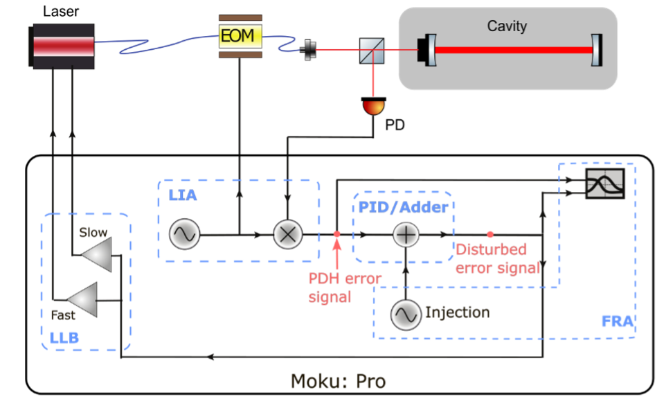
Figure 3: The experimental setup of characterizing the in-loop disturbance rejection of a laser stabilization system. The disturbance rejection was directly measured and generated using the Frequency Response Analyzer instrument, while the laser is locked to the external reference cavity with the Laser Lock Box for Moku:Pro. The injection or adder is achieved by using the PID Controller instrument with 0 dB proportional gain setting.
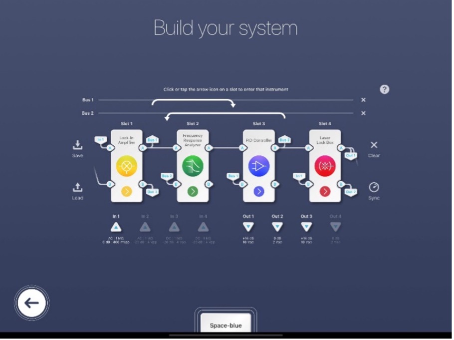
Figure 4: Moku:Pro configuration in Multi-Instrument Mode. Note as the four slots are completely independent of each other, the order of the instruments added into the slots does not matter.
The disturbance is injected after the error signal demodulation but before propagating to the controller. Thus, we separated the laser locking procedure into two separate processes: the Lock-in Amplifier to generate the modulation signal to the electro-optic modulator (EOM) through Out 1 and to demodulate the error signal; and the Laser Lock Box, which skipped the demodulation process and only provided the servo or control signal back to the laser. Out 2, which was from the fast PID controller in the Laser Lock Box, was then connected directly to the laser’s piezo to finely actuate laser frequency, and Out 3 was connected to the laser’s temperature control.
At the same time, we measured the closed-loop disturbance rejection with the Frequency Response Analyzer instrument, where it generated a swept sinusoidal excursion and injected into the in-loop signal (In 1) by using a PID Controller instrument as an adder. To achieve this summing junction, we configured the PID Controller as an adder by setting an input matrix as \([(1, 1), (0,1)]\) and the proportional gain to 0 dB. The output of the adder was split into two paths, one providing the error signal for the Laser Lock Box and the other connected to the Channel B of the Frequency Response Analyzer to measure the closed-loop frequency response. Channel A recorded the in-loop frequency noise before injecting the sinusoidal wave.
The Laser Lock Box supplied the servo action. The PDH error signal was monitored by a ramp scan, then we adjusted the slow temperature offset to bring the cavity resonance close to the middle of the scanning range. The integrator saturation was then switched on to avoid over-compensation before the stabilizing the system. We then selected the zero-crossing point of the carrier as the locking point and engaged the lock by using the “Lock Assist” function, which engages the fast PID controller. Lastly, we disabled integrator saturation to enable the full integrator for more gain at low frequencies. Find the detailed explanation of the Laser Lock Box here.
After we successfully locked the laser frequency to the cavity, we switched the instrument of interest to the Frequency Response Analyzer, where the measurement was configured as (In ÷ Out) with a sufficiently small output signal (5 mVpp) on both channels. By sweeping the frequency source across the frequency range of interest, we generated the transfer functions.
Experimental result
Observe the measurement result in Figure 5.
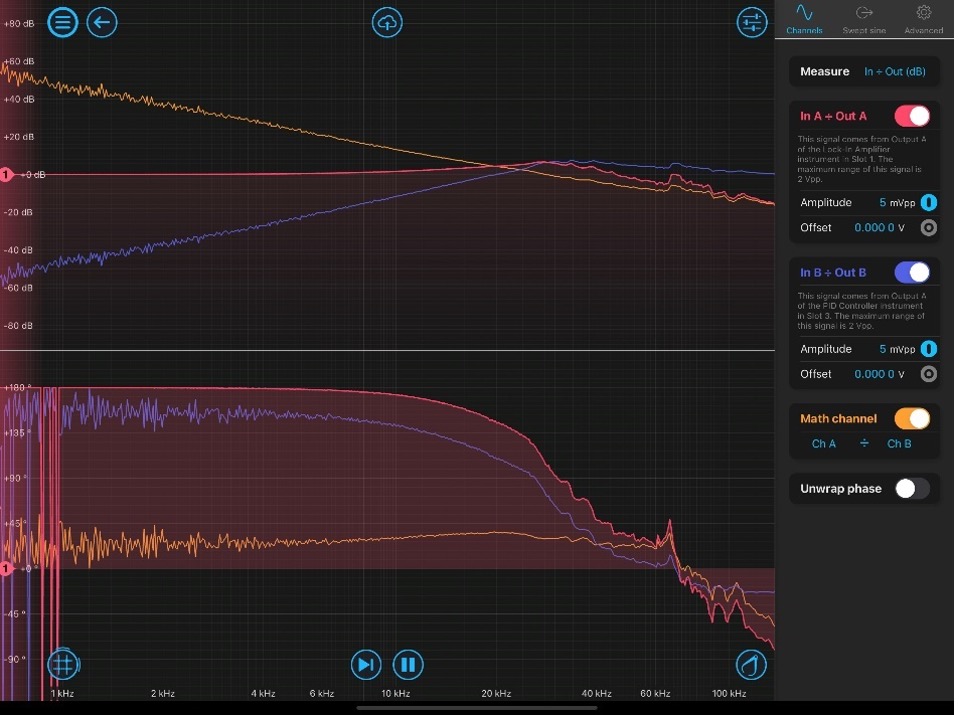
Figure 5: The measured transfer functions, showing overall closed-loop response (red), closed-loop disturbance rejection (blue), and computed open-loop gain of the laser locking system (orange). The unity gain frequency of the disturbance rejection is approximately 24 kHz.
The red trace shows the measured complimentary transfer function (Equation 7), and the blue trace shows the disturbance rejection (Equation 6). By using the math channel (ChA ÷ ChB), we could dynamically calculate the open loop transfer function, shown as the orange trace in Figure 5. From the blue trace (or the orange trace), one can see that the locking loop has a unity gain frequency of up to ~24 kHz with a phase margin slightly more than 90 degrees. The locking bandwidth limit in this system comes from the mechanical resonance of the PZT. From the plots, we can see that there is a mechanical resonance at ~63kHz. Thus, further pushing the system to an even higher gain might excite the resonance oscillation, which may result in positive feedback at this particular frequency point and destabilize the system.
In addition, from the open-loop response (orange trace) we can see the low frequency gain reaches 60 dB. This echoes with the -60 dB perturbations suppression in blue trace and indicates the Laser Lock Box instrument can provide adequate servo gain to sufficiently suppress laser frequency noise and hold a stable lock.
Summary
The flexible field-programmable gate array (FPGA)-based approach of Moku:Pro addresses many of the shortcomings of traditional fixed-function test and measurement hardware. The FPGA-based architecture provides the ability to dynamically switch between instruments. It also provides the ability to use multiple instruments simultaneously, such as characterizing the laser locking loop transfer function with the Frequency Response Analyzer while maintaining a stable lock with the Laser Lock Box. Multi-Instrument Mode makes the process of optimizing the loop configuration much more straightforward and efficient. The intuitive user interface dramatically reduces the complexity of the experimental setup, providing a more accessible and flexible solution.
Moreover, though this application note shows an example utilizing the PDH locking scheme, this method of verifying the control loop response applies to other locking techniques such as DC locking, fringe-side locking, and tilt locking, which open a broad range of practical applications in the laser frequency stabilization field.
Acknowledgements
We would like to thank Andrew Wade, Kirk McKenzie, and The Australian National University for providing us the details of their experiment, explanation of the use of Moku:Pro, and feedback. The experiment at the ANU was supported by the ARC Centre of Excellence for Gravitational Wave Discovery.
References
[1] Doyle, J. C., Francis, B. A., and Tannenbaum, A. R. (2013). Feedback control theory. Courier Corporation.
[2] Black, E.D., 2001. An introduction to Pound–Drever–Hall laser frequency stabilization. American journal of physics, 69(1), pp.79-87.
Questions or comments?
Contact Liquid Instruments Support.